Download
1 / 79
961 likes | 1.77k Vues
Nuclear Magnetic Resonance (NMR) Data Protein–Protein Docking. Presented by: Nivya Papakannu ECE Department, UMASS Amherst. Overview:. Introduction to protein structure Peptide (protein) sequences Primary, Secondary, Tertiary and Quaternary structures. Introduction to NMR

E N D
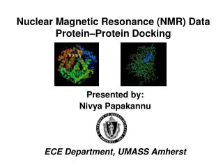
Nuclear Magnetic Resonance (NMR) Data Protein–Protein Docking Presented by: Nivya Papakannu ECE Department, UMASS Amherst
Overview: • Introduction to protein structure • Peptide (protein) sequences • Primary, Secondary, Tertiary and Quaternary structures. • Introduction to NMR • Protein-Protein Interaction. • Mapping Protein-Protein Interactions in Solution by NMR Spectroscopy • Nuclear Overhauser Effect (NOE) • Chemical shift • Titrations with NMR
Overview: • Fast Mapping of Protein-Protein Interfaces by NMR Spectroscopy(chemical shifts and unassigned NMR Data) • Residual Dipolar Coupling • Structures of Protein-Protein Complexes Are Docked Using Only NMRRestraints from Residual Dipolar Coupling and Chemical Shift Perturbations • Other NMR Methods • High-throughput inference of protein–protein interfaces from unassigned NMR data • Summary
PEPTIDES: • Peptides (and proteins) are composed of amino acids interlinked by amide bonds. • Amides are made by condensing together a carboxylic acid and an amine: • a -COOH, which is a carboxyl group (acidic). • a -NH2, which is an amino group (basic). • an -H hydrogen. • a residue R which varies depending on the amino acid. • Any number of amino acids can be joined together to form peptides of any length. • The peptide has a "backbone" and side-chains. The backbone atoms consist of the peptide amide units and the carbons; the side-chains consist of the remaining atoms in the molecule (i.e. the "R" groups of each amino acid):
Proteins: • Proteins are not linear molecules as suggested when we write out a "string" of amino acid sequence, -Lys-Ala-Pro-Met-Gly- etc., for example. • This "string" folds into an intricate 3-D structure, unique to each protein .It is this 3-D Structure that allows proteins to function. • To understand the details of protein functions, we must understand the protein structure. • The Protein structure is broken down into four levels: • Primary Structure refers to ”linear" sequence of amino acids. • Secondary structure is the local spatial arrangement of a polypeptide’s backbone atoms without regard to the conformations of its side chains. • Tertiary structure refers to the three-dimensional structure (global folding) of an entire (single) polypeptide. • Quaternary structure involves association of two or more polypeptide chains, loosely referred to as subunits (refers to the spatial arrangement of the subunits).
Primary Structure of Protein: • Proteins, like peptides, are composed of amino acids joined together via amide linkages. • The only difference between peptides, polypeptides and proteins is the number of amino acid residues in the chain. • Generally, peptides are small 10 or 20 residues; • polypeptides might range up to 50 or 60 residues, with anything larger considered a protein. • Primary structure is sometimes called the "covalent structure" of proteins because, with the exception of disulfide bonds all of the covalent bonding within proteins defines the primary structure. • In contrast, the higher orders of protein structures (i.e. secondary, tertiary and quaternary) involve mainly non-covalent interactions. Primary Structure
Secondary Structure of protein: • Local spatial arrangement of a polypeptide’s backbone atoms without regard to the conformations of its side chains. • The most common secondary structure elements in proteins are the alpha-helix and the Beta-sheet. Alpha-helix: • Right-handed; it turns in the direction that the fingers of a right hand curl when its thumb points in the direction that the helix rises. • The alpha helix has 3.6 residues per turn and a pitch(the distance the helix rises along its axis per turn) of 5.4 Å. • The alpha helices of proteins have an average length of ,12 residues, which corresponds to over three helical turns, and a length of ,18 Å. • Stabilized by hydrogen bonds between the carbonyl oxygen of one amino acid and the backbone nitrogen of a second amino acid located four positions away. • Amino acid side chains project outward and downward from the helix to avoid interference with the polypeptide backbone and with each other.
Beta-Sheet: • Stabilized by hydrogen bonds between the carbonyl oxygen of an amino acid in one strand and the backbone nitrogen of a second amino acid in another strand. (hydrogen bonding occurs between neighboring polypeptide chains rather than within one as in alpha helix) • Beta sheets can be either parallel or anti-parallel. • Anti-parallel beta sheet - neighboring hydrogen-bonded polypeptide chains run in opposite directions. • Parallel beta sheet - hydrogen-bonded chains extend in the same direction. • Beta Sheets in proteins contain 2 to greater than12 polypeptide strands, with an average of 6 strands. • Each strand may contain up to 15 residues, the average being 6 residues.
Tertiary Structure of protein: • The tertiary structure of a protein describes the folding of its secondary structural elements and specifies the positions of each atom in the protein, including those of its side chains. • The atomic coordinates of these structures are deposited in a database known as the Protein Data Bank (PDB) which allows the tertiary structures of a variety of proteins to be analyzed and compared. • The common features of protein tertiary structure reveal much about the biological functions of the proteins and their evolutionary origins. • Structures are determined through X-ray crystallographic or nuclear magnetic resonance (NMR) studies. • Amino acid side chains in globular proteins are spatially distributed according to their polarities: • Non-polar amino acids are "hidden" within the structure, out of contact with the aqueous solvent (hydrophobic). • Charged polar residues are exposed on the outer surface, in contact with the aqueous solvent (hydrophilic). • Uncharged polar groups are usually on the protein surface but also occur in the interior of the molecule. When buried in the protein, the formation of a hydrogen bond “neutralizes” their polarity.
Certain groupings of secondary structural elements,called supersecondary structures or motifs, occur in many unrelated globular proteins: • Most common form of supersecondary structure is the bab-motif, in which an a-helix connects two parallel strands of a b-sheet. • Another common supersecondary structure, the b-hairpin motif, consists of anti-parallel strands connected by relatively tight reverse turns • An aa-motif, two successive anti-parallel a-helices pack against each other with their axes inclined. • Extended b-sheets often roll up to form bb barrels. • Motifs may have functional as well as structural significance. For example, a babab unit, in which the b strands form a parallel sheet with helical connections, often acts as a nucleotide binding site. In most proteins that bind dinucleotides two such babab units combine to form a motif known as a dinucleotide-binding fold.
Quaternary Structure of Protein: • Consists of more than one polypeptide chain with multi subunits. • Usually, each polypeptide within a multi-subunit protein folds more-or-less independently into a stable tertiary structure and the folded subunits then associate with each other to form the final structure. • Stabilized mainly by non-covalent interactions; all types of non-covalent interactions like hydrogen bonding, Vander walls interactions and ionic bonding, are involved in the interactions between subunits. • Hemoglobin is one example of a multi-subunit protein. It has an a2b2 structure consisting of four polypeptides, two alpha subunits and two beta subunits.
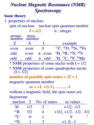
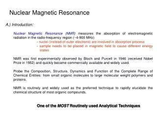
Nuclear Magnetic Resonance (NMR) NMR is a physical phenomenon based upon the magnetic property of an atom's nucleus. NMR studies a magnetic nucleus, like that of a hydrogen atom, by aligning it with an external magnetic field and perturbing this alignment using an electromagnetic field. The response to the field (the perturbing), is what is exploited in NMR spectroscopy. NMR Data:
Bio-molecular structure determination • Structure/imaging from molecules to animals
History of nuclear magnetic resonance • 1946 Bloch, Purcell First nuclear magnetic resonance • 1955 Solomon NOE (nuclear Overhauser effect) • 1966 Ernst, Anderson Fourier transform NMR • 1975 Jeener, Ernst Two-dimensional NMR • 1985 Wüthrich First solution structure of a small protein • from NOE-derived distance restraints NMR is about 25 years younger than X-ray crystallography • 1987/8 3D NMR + 13C, 15N isotope labeling • 1996/7 New long-range structural parameters: - residual dipolar couplings (also: anisotropic diffusion) - cross-correlated relaxation, TROSY (molecular weight > 100 kDa) • 2003 First solid-state NMR structure of a small protein Nobel prizes • 1952 Physics Bloch (Stanford), Purcell (Harvard) • 1991 Chemistry Ernst (ETH) • 2002Chemistry Wüthrich (ETH) • 2003Medicine Lauterbur (Urbana), Mansfield (Nottingham)
Why bio-molecular NMR? • Structure determination of bio-macromolecules # no crystal needed, native-like conditions # nucleic acids: difficult to crystallize, affected by crystal packing • Ligand binding and molecular interactions in solution # NMR fingerprint - with residue/amino acid resolution !!! • Characterization of dynamics and mobility # conformational dynamics ↔ enzyme turnover, kinetics, folding • Molecular weight: X-ray: >200 kDa, NMR < 50-100 kDa. • NMR and X-ray crystallography are complementary
NMR: nuclear spins, magnetic moments and resonance nuclear magnetic dipole A nuclear spin of I > 0 is associated with a magnetic dipole moment µ= γL
Nuclear Magnetic Resonance • Radio frequency pulses Induce resonance by applying an external magnetic field that oscillates with the precession frequency of the spins (radio frequencies: MHz)
Energy levels - why do we need a BIG magnet? • Spins in the α (up) and β (down) states populate the energy levels according to a Boltzmann distribution. • This leads to a small macroscopically observable magnetization along the z-axis Mz (parallel to B0). • No x- or y-magnetization is observed since the spin vectors are not phase coherent, • i.e. they precess independently from each other around B0, the x, y components average to zero • The energy difference between the two states scales with the magnetic field strength B0 • A larger population difference resulting from this yields more nuclear magnetization!
Protein-Protein Interactions: • The study of protein interactions has been vital to the understanding of how proteins function within the cell. Protein A Protein B There are two classes of protein docking: a) Protein-Protein b) Protein-Ligand
Mapping Protein-Protein Interactions in Solution by NMR Spectroscopy
NMR for protein-protein interactions Is it desirable to use NMR for studying protein-protein interactions? • To understand protein-protein interactions is very important for biochemical processes in living organisms. • We need to know the fine details of the interface in protein complexes to understand how life is encoded and how diseases can be cured. • Individual structures do not disclose where the interactions in the complexes take place because many proteins adapt their conformations dramatically to improve the fit. • Resolving the structures of the complexes poses a great challenge for researchers though high resolution individual structures are available. • NMR is very well suited for the study of especially weak protein-protein interactions (i.e. non-covalent interactions), as no crystallization is required. • Scientists have used different NMR techniques to resolve these complex structures.
Nuclear Overhauser Effect (NOE) • This is a special kind of NMR experiment that can be done in 1D or in 2D. • It also gives information about how far apart the different nuclei are from the irradiated nuclei through the 1/r6 relation of the distance between the nuclei to the intensity of the NOE signal.
Nuclear Overhauser Effect: • NOE is an unambiguous way of mapping bio-macromolecular interactions. • A full three-dimensional structure of the complex is determined, using many precise NOE-derived distance constraints between the two interacting partners. • This method is only applicable when the interaction between the molecules is relatively tight.
Nuclear Overhauser Effect: • A powerful method to obtain the intermolecular NOE is the isotope-edited NOE. • Requires that the two interacting macromolecules should have different isotopic labeling patterns. • For instance, one partner has no labeling (i.e., 1H, 14N, 12C) while the other is labeled with stable isotopes, e.g., 1H, 15N, 12C or 1H, 15N, 13C or sometimes even 1H, 2H,15N,13C. Principle: • Distinguishes between protons residing on labeled and unlabeled macro molecules which is an essential ingredient to map the structures. • The isotope editing method is very well suited for the study of labeled proteins and unlabeled nucleic acids.
Cross Saturation • Obtains low-resolution, but gives highly relevant, interface information quickly. • Governed by the same physical processes as the NOE experiment. • Donating partner protein is not labeled, while the observed protein is per-deuterated and 15N-labeled, but its amide deuterons are exchanged back to protons. • Cross-relaxation carries the saturation from the donor to the acceptor protein amide protons, where it is detected using a 15N-1H HSQC or, for larger proteins, 15N-1H TROSY. • Those acceptor 15N-1H cross-peaks that change in intensity upon the donor saturation are very likely to be close to the intermolecular interface.
Cross Saturation: • This experiment is robust because only protons close to the interface will “light up”, even if long-range conformational changes occur. Advantage of cross saturation over NOE: • Because of its experimental simplicity, the method can be widely applied. Disadvantage: • NOE-based methods work only when complexes are relatively tight . Reason: Weaker complexes are best described by an ensemble of interconverting structures, for which the concentrations of the individual structures are too small to give rise to detectable NOEs. • The cross-saturation experiment promises to be more sensitive for weaker interactions than the two- or three-dimensional isotope-edited NOE, because longer magnetization transfer times can be used.
Chemical Shift Perturbation Mapping • Chemical shift perturbation is the most widely used NMR method to map protein interfaces. • In this technique the 15N-1H HSQC spectrum of one protein is monitored when the unlabeled interaction partner is titrated in, and the perturbations of the chemical shifts are recorded. • The interaction causes environmental changes on the protein interfaces and, hence, affect the chemical shifts of the nuclei in this area.
Chemical Shift Perturbation Mapping: • Chemical shift perturbations are very sensitive to subtle effects: • Generally, Shift perturbation measurements just yield the locations of the interfaces on the individual binding partners. It is then still unknown how the partners interact on an atom-to-atom basis. Disadvantage: • In some cases, the entire protein may change conformation, and all shifts may be affected and perturbation fails as a mapping.
Titrations with NMR • Titrations with NMR allows affinity estimation, stoichiometry and kinetics of binding apart from mapping of the interface. • How the chemical shifts of the labeled protein change during the titration is determined by the kinetics of the interaction. • If the complex dissociation is very fast, there is, only a single set of resonances whose chemical shifts are the fractionally weighted average of the free and bound chemical shifts. • This regime is referred to as fast chemical exchange and is often observed for weaker interactions. • If all two-dimensional trajectories are linear and occur at the same rate, a single binding event is indicated. • If the trajectories for different, resonances occur at a different rate, and/or if they are curved, more than one binding site is implicated.
Titrations with NMR: • If the complex dissociation is very slow, one observes one set of resonances for the free protein and one set for the bound protein. During the titration, the “free set” will disappear and will be replaced by the bound set. • This regime is referred to as slow chemical exchange. • In the intermediate chemical exchange case, the frequencies of the changing resonances become poorly defined, and extensive kinetic broadening sets in.
Fast Mapping of Protein-Protein Interfaces by NMR Spectroscopy
NMR allows the study of protein interaction in solution. • Major problem in NMR: - assignment of data before using the results from the NMR spectra. Example: NOE NMR data provides interatomic distance restraints; in order to use these distance restraints in structure determination, we must first assign each restraint to a pair of nuclei in the protein • The assignment is typically done manually and is time consuming. Example: E1N–HPr complex required 2 years of data analysis.
Ability of Mapping through NMR • Advantage of NMR: - Ability to map interfaces efficiently. • A prerequisite for using the chemical shift NMR mapping method, is that the assignment of the nuclei showing chemical shift changes be known. • Here a combinatorial approach was used to map the interface without chemical shift assignments.
Ability of Mapping through NMR • The method is based on preparing several protein samples, each one selectively 15N labeled with one particular amino acid. • The peaks of shifted amino acids of a certain type can be identified. • Combined results, from several differently labeled samples allows to define the minimum number of a certain type of amino acid located in the interface. • Comparison of this list with the known structure of the protein is then used to identify the interface (Figure 1).
Ability of Mapping through NMR • This approach is divided into two phases: - 1) Identify amino acid types with low abundance in the sequence. The combination of data from the rare residues allows us to identify the location of the binding site. -2) Use more common residues to characterize the extent and shape of the interface.
Here in nNOS PDZ domain was studied. Five lysines, four phenylalanines, two histidines, and one tyrosine as initial probes to identify the site of the interface. 15N-lysine labeled nNOS PDZ was titrated with unlabeled PSD-95 PDZ2. Two changes in the spectrum occurred. • One peak disappeared while another peak appeared, characteristic of a complex in slow exchange. • Two other peaks exhibited spectral broadening, characteristic of a complex in intermediate exchange. • This shows 2 distinct interfaces exist. • To distinguish these two interfaces, - Binding site exhibiting slow exchange termed “primary” - Site exhibiting intermediate exchange - “secondary”.
Ability of Mapping by NMR • From the combinatorial approach makes lysine most likely candidate for the primary binding interface. • To further investigate the interface, we labeled the nNOS with 15N-tyrosine, histidine, and phenylalanine. • The results predict that the primary binding site contains at least one lysine, one histidine, and two phenylalanines, but does not contain tyrosine. • The secondary binding site contains two lysines, one tyrosine, no histidines, and one phenylalanine. • Thus mapping for this complex was carried out.
(A) shows the [15N,1H]-HSQC spectrum of the free lysine-labeled PDZ domain from nNOS with five peaks, corresponding to the five lysines. (B) shows the spectrum of a sample in which 50% of the nNOS PDZ domain molecules are in complex with the PDZ2 domain from PSD-95. (C) shows a spectrum of a 1:1 complex of both PDZ domains. (D) His are magenta, Lys are red, Phe are green, and Tyr are gold. (E). Arg are red, His are magenta, Met are cyan, Phe are green, and Tyr are gold. In summary, 2 His, 2 Tyr, 1 Phe, 1 Met, and no Arg were seen to be involved in the primary interface, and 1 His, 1 Tyr, 1 Arg, and neither Phe nor Met were involved in the secondary interface.
Long-range information in NMR • a traditional weakness of NMR is that all the structural restraints are short-range in nature (in terms of distance, not in terms of the sequence), i.e. NOE restraints are only between atoms <5 Å apart, dihedral angle restraints only restrict groups of atoms separated by three bonds or fewer • over large distances, uncertainties in short-range restraints will add up--this means that NMR structures of large, elongated systems (such as B-form DNA, for instance) will be poor overall even though individual regions of the structure will be well-defined. long-range structure bad to illustrate this point, in the picture at left, simulated nOe restraints were generated from the red DNA structure and then used to calculate the ensemble of black structures best fit superposition done for this end short-range structure OK Zhou et al. Biopolymers (1999-2000) 52, 168.