Applied NWP
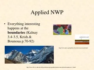
Applied NWP. How do we “shoehorn” the filtered governing equations into the computer weather forecast model? (Kalnay 3.1-3.3.5 & 2.6, Krish.& Bounoua Chap. 2). http://www.thetiecoon.com/sh3.html. Go to: http://www.meted.ucar.edu/nwp/pcu1/ic2/index.htm for more information. Applied NWP.

Applied NWP
E N D
Presentation Transcript
Applied NWP • How do we “shoehorn” the filtered governing equations into the computer weather forecast model? (Kalnay 3.1-3.3.5 & 2.6, Krish.& Bounoua Chap. 2) http://www.thetiecoon.com/sh3.html Go to: http://www.meted.ucar.edu/nwp/pcu1/ic2/index.htm for more information
Applied NWP REVIEW… • As a result of computer limitations, we have to somehow simplify these,… …our governing equations.
Applied NWP • Understanding how we “shoehorn” a simplified version of our governing equations into our computer weather forecast model… …requires a mathematics review.
Applied NWP • Derivatives • Taylor Series Expansions • Partial Differential Equations (PDEs) f (x) http://www.math.ucdavis.edu/~kouba/CalcOneDIRECTORY/graphingdirectory/Graphing.html x
Applied NWP • DERIVATIVES* • at (x, f (x)) the slope m of the graph of y = f (x) is equal to the slope of its tangent line at (x, f(x)), and is determined by the formula provided the limit exists. f (x) x *(Larson and Hostetler, 1982, p.101)
Applied NWP • DERIVATIVES* • The limit is called the derivative of f at x (provided the limit exists). f (x) x *(Larson and Hostetler, 1982, p.101)
Applied NWP DERIVATIVES • Activity- code word- Mimetroupe zonal wind from east or west? u(x) EX: Let, zonal wind from east or west? x
Applied NWP • DERIVATIVES • In our previous activity we used an expression for the zonal wind component that was a continuous function [we knew u(x) at every ‘x’ location] • Is this realistic in practice? x
Applied NWP • DERIVATIVES • No! • Due to computer limitations, we can only represent the atmosphere in our model at regularly-spaced intervals (grid points) Dx does NOT approach 0 o o o o o o o x
Applied NWP • Taylor Expansion • Knowing the atmosphere in our model at regularly-spaced intervals (grid points separated by a distance “Dx”) forces us to obtain derivatives of u(x) using finite differences o o o o o o o x To the board!! http://www.surfboardcollectors.com/
Applied NWP • And now for another activity… http://csep10.phys.utk.edu/astr161/lect/history/newtongrav.html • Activity- code word- Mimetroupe2
Applied NWP • Up to now we have been assuming that the zonal wind component [u] has only been a function of the “x” (east-west) direction • Clearly this is an oversimplification [bummer!] • In reality, u is a function of x, y, and z, [u(x,y,z)] so that the change of u in the x, y, and z directions are represented by a partial derivative… [example given is for the gradient of u, which is a vector]
Applied NWP • A common mathematical operator in meteorology is the horizontal Laplacian: (which is NOT a vector) http://www-groups.dcs.st-and.ac.uk/~history/Mathematicians/Laplace.html
Applied NWP • Finite difference forms of the horizontal Laplacian, using Taylor’s expansion of the functions u(x+/-h, y+/-h) about (x,y), where h is the horizontal grid point spacing: (second order accuracy)
Applied NWP • Finite difference forms of the horizontal Laplacian, using Taylor’s expansion of the functions u(x+/-h, y+/-h) about (x,y), where h is the horizontal grid point spacing: (fourth order accuracy)
Applied NWP • Another common mathematical operator in meteorology is the horizontal Jacobian: (which is NOT a vector) http://www-groups.dcs.st-and.ac.uk/~history/Mathematicians/Jacobi.html
Applied NWP • The horizontal Jacobian is often associated with equations having conserved quantities. Application of finite differencing to such equations can introduce errors that lead to non-conserved quantities. Caution must be made so that errors introduced by the differencing method will not alter the conservation principles. Barotropic absolute vorticity equation, where y is the geostrophic streamfunction and variables a and represent the absolute and relative vorticity, respectively.
Applied NWP • Arakawa (1966) horizontal Jacobian of second order accuracy: Krishnamurti and Bounoua (1996)
Applied NWP • Spatial derivatives give us a view into the atmospheric structure at a snapshot in time • But we want to know “What will be the structure tomorrow?” • Time derivatives!!! http://www.ebay.com/
Applied NWP • Let’s start out with a “simple” linear equation: Before getting into the numerics, what is this zonal momentum equation telling us? (think Newton)
Applied NWP • Assume that “c” is a constant and that: where A, k, and n are also constant. Given this information, what must be the value of “c”? To the board!!
Applied NWP • Given this form of the zonal wind component, what do we know about the behavior of the amplitude of the zonal wind? • Activity- code word- Mimetroupe3
Applied NWP • If we were to find that, after implementing our new finite difference scheme, the amplitude of the zonal wind was found to change with time, what might we conclude? UGH!! Something is WRONG!!
Applied NWP • Stability of the numerical scheme for this simple linear equation is defined as, • Stable if |r | < 1 • Neutral if |r | = 1 • Unstable if |r | > 1, where is an amplification factor
Applied NWP • Partial differential equations (PDEs) • Second order linear PDEs are classified into three types depending on the sign of b 2 – ag. Equations are hyperbolic, parabolic or elliptic if the sign is positive, zero, or negative, respectively.
Applied NWP • Examples • Wave equation (hyperbolic) vibrating string http://www.warwickbass.com/basses/streamer_ct.html http://www.cs.princeton.edu/~mj/string.html http://colos1.fri.uni-lj.si/~colos/COLOS/EXAMPLES/XDJ/VSTRING/Vstring.html
Applied NWP • Examples • Advection equation (first order PDE, hyperbolic) http://www.advection.net/
Applied NWP • Examples • Diffusion equation (parabolic) heated rod http://heatex.mit.edu/HeatexWeb/ExtendedSurfaceHeatTransfer.pdf
Applied NWP • Examples • Laplace’s or Poisson’s equations (elliptic) steady state temperature of a plate http://www.galasource.com/prodDetail.cfm/20170,Gold%20Beaded%20Lacquer%20Charger%2012%22,MX2
Applied NWP • Well-posed problem • Must specify proper initial conditions and boundary conditions • Too few solution will NOT be unique • Too many no solution • “just right” accurate solution if specified at the right place and time http://pubs.usgs.gov/publications/msh/catastrophic.html
Applied NWP • Ill-posed problem • Small errors in the initial/boundary conditions will produce huge errors in the solution • Computer weather forecast model will “blow up” http://pubs.usgs.gov/publications/msh/catastrophic.html
Applied NWP • One method of solving simple PDEs is the method of separation of variables, but unfortunately in most cases it is not possible to use it • hence the need for numerical models! http://heatex.mit.edu/HeatexWeb/ExtendedSurfaceHeatTransfer.pdf
Applied NWP • Hyperbolic and parabolic PDEs are initial value or marching problems • The solution is obtained by using the known initial values and marching or advancing in time wave or advection equation, a hyperbolic equation diffusion equation, a parabolic equation
Applied NWP • Example • Upstream Scheme of the finite difference equation (FDE) of the wave or advection equation PDE
Applied NWP • Two questions must be asked • Is the FDE consistent with the PDE? • Will the solution of the FDE converge to the PDE solution as Dx0 and Dt0? PDE
Applied NWP • Two questions must be asked • Is the FDE consistent with the PDE? • Will the solution of the FDE converge to the PDE solution as Dx0 and Dt0? • FDE is consistent with PDE if, in limit Dx0 and Dt0 the FDE coincides with the PDE • How to verify this? • Substitute U by u in the FDE • Evaluate all terms using a Taylor series expansion centered on point (j,n) • Subtract PDE from FDE To the board!!
Applied NWP • Two questions must be asked • Is the FDE consistent with the PDE? • Will the solution of the FDE converge to the PDE solution as Dx0 and Dt0? Before addressing the second question, we must explore the concept of computational stability
Applied NWP • Computational stability • Ujn+1is interpolated from Ujn and Unj-1 in (a) • Ujn+1is extrapolated from Ujn and Unj-1 in (b) and (c) • Activity- code word- Mimetroupe3
Applied NWP • Computational stability Courant-Friedrichs-Lewy (CFL) condition
Applied NWP • Computational stability* Courant-Friedrichs-Lewy (CFL) condition *an FDE is computationally stable if the solution of the FDE at a fixed time t = nDt remains bounded as Dt0.
Applied NWP • Lax-Richtmyer theorem • Given a properly posed linear initial value problem, and a finite difference scheme that satisfies the consistency condition, then the stability of the FDE is the necessary and sufficient condition for convergence. http://www.convergence2004.org/ We want to make sure that if Dt, Dx are small, then the errors u( j Dx, n Dt) – Ujn (accumulated or global truncation errors at a finite time) are acceptably small.
Applied NWP • Computational stability for the FDE of the parabolic diffusion equation PDE
Applied NWP • Unfortunately, the previous methods for determining stability work for only a few cases • von Neumann stability criterion; a stability criterion having much wider application http://www-groups.dcs.st-and.ac.uk/~history/Mathematicians/Von_Neumann.html
Applied NWP • von Neumann stability criterion; r is the amplification factor and the term O(Dt) allows bounded growth (if it arises from a physical instability) http://www-sccm.stanford.edu/Students/witting/ctei.html But how do we determine the amplification factor? To the board!!
Applied NWP • Up to now we have been concerned with |r| > 1 • However, |r| << 1 can be a problem within a computer weather forecast model, as well
Applied NWP • The amplification factor r indicates how much the amplitude of each wavenumber will decrease or increase with each time step. • The upstream scheme decreases the • amplitude of all wave components • It is a very dissipative FDE (it has • strong “numerical diffusion”)
Applied NWP • Other time scheme examples… • Matsuno (Euler-backward) scheme • Leapfrog scheme
Applied NWP • Leapfrog scheme; two solutions • “legitimate” weather mode • computational mode* *Arises because the leapfrog scheme has three time levels. http://www.leapfrog.com/
Applied NWP • Leapfrog scheme; two unique problems • needs a special initial step to get to the first time level (n=1) from the initial conditions (n=0) before it can get started • for non-linear examples, it has a tendency to increase the amplitude of the computational mode with time A time filter (e.g. Robert-Asselin) is applied to solve problem #2
Applied NWP http://www.atmos.ucla.edu/~fovell/AS180/dispersion.html • Leapfrog scheme; two unique problems • needs a special initial step to get to the first time level (n=1) from the initial conditions (n=0) before it can get started • for non-linear examples, it has a tendency to increase the amplitude of the computational mode with time A time filter (e.g. Robert-Asselin) is applied to solve problem #2