Texture Mapping
Texture Mapping. CSE167: Computer Graphics Instructor: Steve Rotenberg UCSD, Fall 2005. Texture Mapping. Texture mapping is the process of mapping an image onto a triangle in order to increase the detail of the rendering

Texture Mapping
E N D
Presentation Transcript
Texture Mapping CSE167: Computer Graphics Instructor: Steve Rotenberg UCSD, Fall 2005
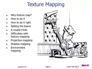
Texture Mapping • Texture mapping is the process of mapping an image onto a triangle in order to increase the detail of the rendering • This allows us to get fine scale details without resorting to rendering tons of tiny triangles • The image that gets mapped onto the triangle is called a texture map or texture and is usually a regular color image
Texture Map • We define our texture map as existing in texture space, which is a normal 2D space • The lower left corner of the image is the coordinate (0,0) and the upper right of the image is the coordinate (1,1) • The actual texture map might be 512 x 256 pixels for example, with a 24 bit color stored per pixel
Texture Coordinates • To render a textured triangle, we must start by assigning a texture coordinate to each vertex • A texture coordinate is a 2D point [txty] in texture space that is the coordinate of the image that will get mapped to a particular vertex
Texture Mapping (1,1) v1 t1 v0 y t2 t0 v2 (0,0) x Texture Space Triangle (in any space)
Vertex Class • We can extend our concept of a Model to include texture coordinates • We can do this by simply extending the Vertex class: class Vertex { Vector3 Position; Vector3 Color; Vector3 Normal; Vector2 TexCoord; public: void Draw() { glColor3f(Color.x, Color.y, Color.z); glNormal3f(Normal.x, Normal.y, Normal.z); glTexCoord2f(TexCoord.x, TexCoord.y); glVertex3f(Position.x, Position.y, Position.z); // This has to be last } };
Texture Interpolation • The actual texture mapping computations take place at the scan conversion and pixel rendering stages of the graphics pipeline • During scan conversion, as we are looping through the pixels of a triangle, we must interpolate the txty texture coordinates in a similar way to how we interpolate the rgb color and z depth values • As with all other interpolated values, we must precompute the slopes of each coordinate as they vary across the image pixels in x and y • Once we have the interpolated texture coordinate, we look up that pixel in the texture map and use it to color the pixel
Perspective Correction • The scan conversion process usually uses linear interpolation to interpolate values across the triangle (colors, z, etc.) • If we use linear interpolation to interpolate the texture coordinates, we may run into inaccuracies • This is because a straight line of regularly spaced points in 3D space maps to a straight line of irregularly spaced points in device space (if we are using a perspective transformation) • The result is that the texture maps exactly onto the triangle at the vertices, but may warp and stretch within the triangle as the viewing angle changes • This is known as texture swimming and can be quite distracting on large triangles • To fix the problem, we must perform a perspective correct interpolation, or hyperbolic interpolation • This requires interpolating the w coordinate across the triangle and performing a perspective division for each pixel • See page 121 & 128 in the book for more info
Pixel Rendering • Usually, we want to combine texture mapping with lighting • Let’s assume that we are doing vertex lighting and using Gouraud shading to interpolate the lit colors across the triangle • As we render each pixel, we compute the interpolated light color and multiply it by the texture color to get our final pixel color • Often, when we are using texture maps, we don’t need to use vertex colors, and so they are implicitly set to (1,1,1) • The texture map itself usually defines the material color of the object, and it is allowed to vary per pixel instead of only per vertex
Pixel Rendering • Let’s consider the scan conversion process once again and look at how the pixel rendering process fits in • Remember that in scan conversion of a triangle, we loop from the top row down to the bottom row in y, and then loop from left to right in x for each row • As we are looping over these pixels, we are incrementing various interpolated values (such as z, r, g, b, tx, and ty) • Each of these increments requires only 1 addition per pixel, but perspective correction requires 1 an additional divide per pixel and 1 additional multiply per pixel for each perspective corrected value • Before actually writing the pixel, we compare the interpolated z value with the value written into the zbuffer, stored per pixel. If it is further than the existing z value, we don’t render the pixel and proceed to the next one. If it is closer, we finish rendering the pixel by writing the final color into the framebuffer and the new z value into the zbuffer • If we are doing expensive per-pixel operations (such as Phong interpolation & per-pixel lighting), we can postpone them until after we are sure that the pixel passes the zbuffer comparison. If we are doing a lot of expensive per-pixel rendering, it is therefore faster if we can render closer objects first
Tiling • The image exists from (0,0) to (1,1) in texture space, but that doesn’t mean that texture coordinates have to be limited to that range • We can define various tiling or wrapping rules to determine what happens when we go outside of the 0…1 range
y x Tiling (1,1) (0,0) Texture Space
y x Clamping (1,1) (0,0) Texture Space
y x Mirroring (1,1) (0,0) Texture Space
Combinations • One can usually set the tiling modes independently in x and y • Some systems support independent tiling modes in x+, x-, y+, and y-
Texture Space • Let’s take a closer look at texture space • It’s not quite like the normalized image space or device spaces we’ve seen so far • The image itself ranges from 0.0 to 1.0, independent of the actual pixel resolution • It allows tiling of values <0 and >1 • The individual pixels of the texture are called texels • Each texel maps to a uniform sized box in texture space. For example, a 4x4 texture would have pixel centers at 1/8, 3/8, 5/8, and 7/8
Magnification • What happens when we get too close to the textured surface, so that we can see the individual texels up close? • This is called magnification • We can define various magnification behaviors such as: • Point sampling • Bilinear sampling • Bicubic sampling
Magnification • With point sampling, each rendered pixel just samples the texture at a single texel, nearest to the texture coordinate. This causes the individual texels to appear as solid colored rectangles • With bilinear sampling, each rendered pixel performs a bilinear blend between the nearest 4 texel centers. This causes the texture to appear smoother when viewed up close, however, when viewed too close, the bilinear nature of the blending can become noticeable • Bicubic sampling is an enhancement to bilinear sampling that actually samples a small 4x4 grid of texels and performs a smoother bicubic blend. This may improve image quality for up close situations, but adds some memory access costs
Minification • Minification is the opposite of magnification and refers to how we handle the texture when we view it from far away • Ideally, we would see textures from such a distance as to cause each texel to map to roughly one pixel • If this were the case, we would never have to worry about magnification and minification • However, this is not a realistic case, as we usually have cameras moving throughout an environment constantly getting nearer and farther from different objects • When we view a texture from too close, a single texel maps to many pixels. There are several popular magnification rules to address this • When we are far away, a many texels may map to a single pixel. Minification addresses this issue • Also, when we view flat surfaces from a more edge on point of view, we get situations where texels map to pixels in a very stretched way. This case is often handled in a similar way to minification, but there are other alternatives
Minification • Why is it necessary to have special handling for minification? • What happens if we just take our per-pixel texture coordinate and use it to look up the texture at a single texel? • Just like magnification, we can use a simple point sampling rule for minification • However, this can lead to a common texture problem known as shimmering or buzzing which is a form of aliasing • Consider a detailed texture map with lots of different colors that is only being sampled at a single point per pixel • If some region of this maps to single pixel, the sample point could end up anywhere in that region. If the region has large color variations, this may cause the pixel to change color significantly even if the triangle only moves a minute amount. The result of this is a flickering/shimmering/buzzing effect • To fix this problem, we must use some sort of minification technique
Minification • Ideally, we would look at all of the texels that fall within a single pixel and blend them somehow to get our final color • This would be expensive, mainly due to memory access cost, and would get worse the farther we are from the texture • A variety of minification techniques have been proposed over the years (and new ones still show up) • One of the most popular methods is known as mipmapping
Mipmapping • Mipmapping was first published in 1983, although the technique had been in use for a couple years at the time • It is a reasonable compromise in terms of performance and quality, and is the method of choice for most graphics hardware • In addition to storing the texture image itself, several mipmaps are precomputed and stored • Each mipmap is a scaled down version of the original image, computed with a medium to high quality scaling algorithm • Usually, each mipmap is half the resolution of the previous image in both x and y • For example, if we have a 512x512 texture, we would store up to 8 mipmaps from 256x256, 128x128, 64x64, down to 1x1 • Altogether, this adds 1/3 extra memory per texture (1/4 + 1/16 + 1/64…= 1/3) • Usually, texture have resolutions in powers of 2. If they don’t, the first mipmap (the highest res) is usually the original resolution rounded down to the nearest power of 2 instead of being half the original res. This causes a slight memory penalty • Non-square textures are no problem, especially if they have power of 2 resolutions in both x and y. For example, an 16x4 texture would have mipmaps of 8x2, 4x1, 2x1, and 1x1
Mipmapping • When rendering a mipmapped texture, we still compute an interpolated tx,ty per pixel, as before • Instead of just using this to do a point sampled (or bilinear…) lookup of the texture, we first determine the appropriate mipmap to use • Once we have the right mipmap, we can either point sample or bilinear sample it • If we want to get fancy, we can also perform a blend between the 2 nearest mipmaps instead of just picking the 1 nearest. With this method, we perform a bilinear sample of both mips and then do a linear blend of those. This is called trilinear mipmapping and is the preferred method. It requires 8 texels to be sampled per pixel
Mipmapping Limitations • Mipmapping is a reasonable compromise in terms of performance and quality • It requires no more than 8 samples per pixel, so its performance is predictable and parallel friendly • However, it tends to have visual quality problems in certain situations • Overall, it tends to blur things a little much, especially as the textured surfaces appear more edge-on to the camera • The main reason for its problems comes from the fact that the mipmaps themselves are generated using a uniform aspect filter • This means that if a roughly 10x10 region of texels maps to a single pixel, we should be fine, as we would blend between the 16x16 and 8x8 mipmaps • However, if a roughly 10x3 region maps to a single pixel, the mip selector will generally choose the worst of the two dimensions to be safe, and so will blend between the 4x4 and 2x2 mipmaps
Anisotropic Mipmapping • Modern graphics hardware supports a feature called anisotropic mipmapping which attempts to address the edge-on blurring issue • With this technique, rectangular mipmaps are also stored in addition to the square ones. Usually aspect ratios of 2x1 or 4x1 are chosen as limits • In other words, a 512x512 texture with 2x1 anisotropic mipmapping would store mipmaps for: 256x512, 512x256, 256x256, 256x128, 128x256, 128x128… 2x1, 1x2, 1x1 • Regular mipmapping (1x1 aspect) adds 1/3 memory per texture • 2x1 aspect adds 2/3 extra memory per texture • 4x1 aspect adds 5/6 extra memory per texture • Anisotropic mipmapping improves image quality for edge on situations, but the high aspect rectangles are still xy aligned, and so the technique doesn’t work well for diagonal viewing situations • In fact, 4x1 aspect and higher can tend to have noticeably varying blur depending on the view angle. This would be noticed if one was standing on a large relatively flat surface (like the ground) and turning around in place • Anisotropic mipmapping adds little hardware complexity and runtime cost, and so is supported by modern graphics hardware. It is an improvement over the standard technique, but is still not ideal
Eliptical Weighted Averaging • Present day realtime graphics hardware tends to use mipmapping or anisotropic mipmapping to fix the texture buzzing problem • Some high quality software renderers use these methods as well, or enhanced variations • Perhaps the highest quality technique (though not the fastest!) is one called eliptical weighted averaging or EWA • This technique is based on the fact that a circle in pixel space maps to an ellipse in texture space • We want to sample all of the texture that falls within the pixel, however, we will weight the texels higher based on how close they are to the center of the pixel • We use some sort of radial distribution to define how the pixel is sampled. A common choice is a radial Gaussian distribution • Each concentric circle in this distribution maps to a ellipse in texture space, so the entire radial Gaussian distribution of a pixel maps to a series of concentric ellipses in texture space • With the EWA technique, we sample all of the texels, weighted by their location in this region • This technique represents the theoretically best way to sample the texture, but is really only useful in theory, as it can be prohibitively expensive in real situations • There are some advanced mipmapped EWA techniques where the EWA actually performs a relatively small number of samples from mipmapped textures. This method combines the best of both techniques, and offers a fast, high quality, hardware friendly technique for texture sampling. However, it is fairly new and not used in any production hardware that I know of.
Antialiasing • These minification techniques (mipmapping, EWA) address the buzzing/shimmering problems we see when we view textures from a distance • These techniques fall into the broader category of antialiasing techniques, as texture buzzing is a form of aliasing • We will discuss more about aliasing and antialiasing in a later lecture
Basic Texture Mapping • To render a texture mapped triangle, we must first assign texture coordinates to the vertices • These are usually assigned at the time the object is created, just as the positions, normals, and colors • The tx and ty texture coordinates are interpolated across the triangle in the scan conversion process, much like the z value, or the r, g, and b. However, unlike the other values, it is highly recommended to do a perspective correct interpolation for texture coordinates • Once we have a texture coordinate for the pixel, we perform some sort of texture lookup. This will make use of the minification or magnification rules as necessary, and commonly involves looking up and combining 8 individual texels for trilinear mipmapping (min), or 4 texels for bilinear sampling (mag) • This texture color is then usually blended with the interpolated rgb color to generate the final pixel color
Texture Coordinate Assignment • Now that we have seen the basic texture mapping process, let’s look at different ways that we might assign texture coordinates • We could just let the user type in the numbers by hand, but that wouldn’t be too popular, especially for 1000000 vertex models… • More often, we use some sort of projection during the interactive modeling process to assign the texture coordinates • Different groups of triangles can be mapped with different projections, since ultimately, it just ends up as a bunch of texture coordinates • We can think of the texture coordinate assignment process as a similar process to how we though of transforming vertices from 3D object space to 2D image space • In a sense, assigning texture coordinates to 3D geometry is like transforming that 3D geometry into 2D texture space • We can literally use the same mappings we used for camera viewing, but a variety of additional useful mappings exist as well • Often, texture coordinates are assigned in the modeling process, but sometimes, they are assigned ‘on the fly’, frame by frame to achieve various dynamic effects
Orthographic Mapping • Orthographic mappings are very common and simple • We might use this in the offline modeling process to map a brick texture onto the side of a building, or a grass texture onto a terrain • We can also use it dynamically in a trick for computing shadows from a directional light source
Perspective Mapping • Perspective mappings tend to be useful in situations where one uses a texture map to achieve lighting effects • For example, one can achieve a slide projector effect by doing a perspective projection of a texture map on to an object • It is also useful in certain shadow tricks, like the orthographic mapping
Spherical Mapping • A variety of spherical mappings can be constructed, but the most common is a polar mapping • Think of the texture image itself getting mapped onto a giant sphere around our object, much like a map of the earth • The tx coordinate maps to the longitude and the ty coordinate maps to latitude • Then think of this sphere being shrink wrapped down to project onto the object • This technique is useful for mapping relatively round object, such as a character’s head and face
Cylindrical Mapping • The cylindrical mapping is similar to the spherical mapping, and might also be useful for character heads or similar situations
Skin Mappings • A variety of fancy mapping techniques have been developed to wrap a texture around a complex surface • These include • Conformal mappings (mappings that preserve angles) • Area preserving mappings • Pelting • And more…
Environment Mapping • Environment mapping is a simple but powerful technique for faking mirror-like reflections • It is also known as reflection mapping • It is performed dynamically each frame for each vertex, and is based on the camera’s position • Environment mapping is similar to the spherical mapping, in that we start by visualizing a giant sphere centered at the camera, with the texture mapped onto it in a polar fashion • For each vertex, we compute the vector e from the vertex to the eye point. We then compute the reflection vector r, which is e reflected by the normal • We assume that r hits our virtual spherical surface at somewhere, so we use that as the texture coordinate
Environment Mapping n r e
Cube Mapping • Cube mapping is essentially an enhancement to sphere mapping and environment mapping • As both of those techniques require polar mappings, both of them suffer from issues near the actual poles, where the entire upper and lower rows of the image get squashed into a single point • Cube or box mapping uses six individual square texture maps mapped onto a virtual cube, instead of a single texture mapped onto a virtual sphere • The result is that one gets a cleaner mapping without visual problems • It can also save memory, as the total number of texels can often be smaller for equal or better visual quality • It also should run faster, as it only requires some comparison logic and a single division to get the final texture coordainte, instead of inverse trigonometric functions • It also has the advantage in that the six views are simple 90 degree perspective projections and can actually be rendered on the fly!
Solid Textures • It is also possible to use volumetric or solid textures • Instead of a 2D image representing a colored surface, a solid texture represents the coloring of a 3D space • Solid textures are often procedural, because they would require a lot of memory to explicitly store a 3D bitmap • A common example of solid texture is marble or granite. These can be described by various mathematical functions that take a position in space and return a color • Texturing a model with a marble solid texture can achieve a similar effect to having carved the model out of a solid piece of marble
Texture Combining • Textures don’t just have to represent the diffuse coloring of a material- they can be used to map any property onto a triangle • One can also combine multiple textures onto the same triangle through a variety of combination rules • For example, if we shine a slide projector onto a brick wall, we could map the surface with both the brick texture and the projected image • The triangle would have two sets of texture coordinates, and both would be interpolated in the scan conversion process • At the final pixel rendering stage, the textures are combined according to certain rules that can be set up to achieve a variety of effects • We will discuss the concept of texture combining and shaders more in another lecture
Bump Mapping • As we said, a texture doesn’t always have to represent a color image • The technique of bump mapping uses a texture to represent the variable height of a surface • For example, each texel could store a single 8 bit value which represents some variation from a mean height • Bump mapping is used in conjunction with Phong shading (interpolating normals across the triangle and applying the lighting equations per pixel) • The Phong shading provides an interpolated normal per pixel, which is then further perturbed according to the bump map • This perturbed normal is then used for per-pixel lighting • This allows one to use a bump map to fake small surface irregularities that properly interact with lighting • Bump mapping is definitely a hack, as a triangle still looks flat when viewed edge-on. However, it is a very popular technique and can be very useful for adding subtle shading details • State of the art graphics hardware supports Phong shading, bump mapping, and per pixel lighting
Displacement Mapping • The more advanced technique of displacement mapping starts with the same idea as bump mapping • Instead of simply tweaking the normals, the displacement mapping technique perturbs the actual surface itself • This essentially requires dicing the triangle up into lots of tiny triangles (often about 1 pixel in size) • Obviously, this technique is very expensive, but is often used in high quality rendering