Three-Group Illustrative Example of Discriminant Analysis

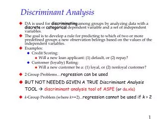
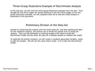
1. Three-Group Illustrative Example of Discriminant Analysis In this exercise, we will work the three-group illustrative example from the text.  Even though the first three stages are almost identical to the first three stages of the two-group illustrative example, we will complete them all so that the whole analysis is presented in this document. Preliminary Division of the Data Set Instead of conducting the analysis with the entire data set, and then splitting the data for the validation analysis, the authors opt to divide the sample prior to doing the analysis.  They use the estimation or learning sample of 60 cases to build the discriminant model and the other 40 cases for a holdout sample to validate the model. To replicate the author's analysis, we will create a randomly generated variable, randz, to split the sample.  We will use the cases where randz = 0 to create the discriminant model. Discriminant Analysis

2. Specify the Random Number Seed Discriminant Analysis

3. Compute the random selection variable Discriminant Analysis

4. Stage One: Define the Research Problem • In this stage, the following issues are addressed: • Relationship to be analyzed • Specifying the dependent and independent variables • Method for including independent variables Relationship to be analyzed The purpose of this analysis is to identify the perceptions of HATCO that differ significantly between firms according to the type of purchasing situation most often faced: New Task, Modified Rebuy, and Straight Rebuy.  From this information, HATCO can develop targeted strategies in each purchasing situation that accentuate its perceived strengths. (Text, page 296) The data set for this analysis is HATCO.SAV. Discriminant Analysis

5. Specifying the dependent and independent variables • The dependent variable is: • X14, Type of Buying Situation, with three categories: 1 = New Task, 2 = Modified Rebuy, 3 = Straight Rebuy • The independent variables are the seven metric perception variables: • X1, Delivery Speed • X2, Price Level • X3, Price Flexibility • X4, Manufacturer Image • X5, Service • X6, Sales Force Image • X7, Product Quality Method for including independent variables Since the purpose of this analysis is to identify the variables which do the best job of differentiating between the three groups, the stepwise method for selecting variables is appropriate. Discriminant Analysis

6. Stage 2: Develop the Analysis Plan: Sample Size Issues • In this stage, the following issues are addressed: • Missing data analysis • Minimum sample size requirement: 20+ cases per independent variable • Division of the sample: 20+ cases in each dependent variable group Missing data analysis There is no missing data in this data set. Minimum sample size requirement: 20+ cases per independent variable With 100 cases and 7 independent variables, we have a ratio of 14 cases per independent variable, close to the suggested ratio of 20 to 1. When we reduce the effective sample size for building the model to 60 cases, we fall to a 9 to 1 ratio; however the authors do not identify this as a problem. Division of the sample: 20+ cases in each dependent variable group In the sample used to build the model, we have 21 cases in the New Task group, 15 cases in the Modified Rebuy group, and 24 cases in Straight Rebuy group.  We do not meet this requirement for the Modified Rebuy group. However, since this a sample problem, we will continue with the analysis. Discriminant Analysis

7. Stage 2: Develop the Analysis Plan: Measurement Issues: • In this stage, the following issues are addressed: • Incorporating nonmetric data with dummy variables • Representing curvilinear effects with polynomials • Representing interaction or moderator effects Incorporating Nonmetric Data with Dummy Variables All of the nonmetric variables have recoded into dichotomous dummy-coded variables. Representing Curvilinear Effects with Polynomials We do not have any evidence of curvilinear effects at this point in the analysis. Representing Interaction or Moderator Effects We do not have any evidence at this point in the analysis that we should add interaction or moderator variables. Discriminant Analysis

8. Stage 3: Evaluate Underlying Assumptions • In this stage, the following issues are addressed: • Nonmetric dependent variable and metric or dummy-coded independent variables • Multivariate normality of metric independent variables: assess normality of individual variables • Linear relationships among variables • Assumption of equal dispersion for dependent variable groups Nonmetric dependent variable and metric or dummy-coded independent variables All of the variables in the analysis are metric or dummy-coded. Discriminant Analysis

9. Multivariate normality of metric independent variables Since there is not a method for assessing multivariate normality, we assess the normality of the individual metric variables. We did the assessment of normality for the metric variables in this data set in the class 6 exercise "Illustration of a Regression Analysis." In that exercise, we found that the tests of normality indicated that the following variables are normally distributed: X1  'Delivery Speed', and X5  'Service'. The following independent variables are not normally distributed:  X2 'Price Level', X3 'Price Flexibility, X4 'Manufacturer's Image', X6 'Sales force Image', and X7 'Product Quality'. X2 'Price Level' is induced to normality by a log and a square root transformation. X7 'Product Quality' is induced to normality by a log and a square root transformation. The other non-normal variables are not improved by a transformation.  Note that this finding does not agree with the text, which finds that X2 'Price Level', X4 'Manufacturer Image', and X6 'Salesforce Image' are correctable with a log transformation. I have no explanation for the discrepancy. We can use include the transformed version of the variables in an additional analysis to see if they improve the overall fit between the dependent and the independent variables. Discriminant Analysis

10. Linear relationships among variables Since our dependent variable is not metric, we cannot use it to test for linearity of the independent variables. As an alternative, we can plot each metric independent variable against all other independent variables in a scatterplot matrix to look for patterns of nonlinear relationships.  If one of the independent variables shows multiple nonlinear relationships to the other independent variables, we consider it a candidate for transformation Discriminant Analysis

11. Requesting a Scatterplot Matrix Discriminant Analysis

12. Specifications for the Scatterplot Matrix Discriminant Analysis

13. The Scatterplot Matrix Blue fit lines were added to the scatterplot matrix to improve interpretability. Having computed a scatterplot for all combinations of metric independent variables, we identify all of the variables that appear in any plot that shows a nonlinear trend. We will call these variables our nonlinear candidates. To identify which of the nonlinear candidates is producing the nonlinear pattern, we look at all of the plots for each of the candidate variables. The candidate variable that is not linear should show up in a nonlinear relationship in several plots with other linear variables. Hopefully, the form of the plot will suggest the power term to best represent the relationship, e.g. squared term, cubed term, etc. None of our metric independent variables show a strong nonlinear pattern, so no transformations will be used in this analysis. Discriminant Analysis

14. Assumption of equal dispersion for dependent variable groups Box's M test evaluates the homogeneity of dispersion matrices across the subgroups of the dependent variable.  The null hypothesis is that the dispersion matrices are homogenous.  If the analysis fails this test, we can request using separate group dispersion matrices in the classification phase of the discriminant analysis to see it this improves our accuracy rate. Box's M test is produced by the SPSS discriminant procedure, so we will defer this question until we have obtained the discriminant analysis output. Discriminant Analysis

15. Stage 4: Estimation of Discriminant Functions and Overall Fit: The Discriminant Functions • In this stage, the following issues are addressed: • Compute the discriminant analysis • Overall significance of the discriminant function(s) Compute the discriminant analysis The steps to obtain a discriminant analysis are detailed on the following screens. We will not produce all of the output provided in the text for two reasons.  First, some of the output can only be obtained with syntax commands.  Second, some of the authors’ analyses are either produced with other statistical software or are computed by hand.  In spite of this, we can produce sufficient output with the menu commands to do a creditable analysis. Discriminant Analysis

16. Requesting a Discriminant Analysis Discriminant Analysis

17. Specifying the Dependent Variable Discriminant Analysis

18. Specifying the Independent Variables Discriminant Analysis

19. Selecting the Cases to Include in the Analysis Discriminant Analysis

20. Specifying Statistics to Include in the Output Discriminant Analysis

21. Specifying the Stepwise Method for Selecting Variables Discriminant Analysis

22. Specifying the Classification Requirement Discriminant Analysis

23. Complete the Discriminant Analysis Request Discriminant Analysis

24. Overall significance of the discriminant function(s) - 1 Similar to multiple regression analysis, our first task is to determine whether or not there is a statistically significant relationship between the independent variables and the dependent variable. We navigate to the section of output titled "Summary of Canonical Discriminant Functions" to locate the following outputs: Recall that the maximum number of discriminant functions is equal to the number of groups in the dependent variable minus one, or the number of variables in the analysis, whichever is smaller. For this problem, the maximum number of discriminant functions is two. In the Wilks' Lambda table, SPSS successively tests models with an increasing number of functions. The first line of the table tests the null hypothesis that the mean discriminant scores for the two possible functions are equal in the subgroups of the dependent variable. Since the probability of the chi-square statistic for this test is less than 0.0001, we reject the null hypothesis and conclude that there is at least one statistically significant function. Had the probability for this test been larger than 0.05, we would have concluded that there are no discriminant functions to separate the groups of the dependent variable and our analysis would be concluded. Discriminant Analysis

25. Overall significance of the discriminant function(s) - 2 The second line of the Wilks' Lambda table tests the null hypothesis that the mean discriminant scores for the second possible discriminant function are equal in the subgroups of the dependent variable. Since the probability of the chi-square statistic for this test is less than 0.0001, we reject the null hypothesis and conclude that the second discriminant function, as well as the first, is statistically significant. Had the probability for this test been larger than 0.05, we would have concluded that there is only one discriminant function to separate the groups of the dependent variable. Our conclusion from this output is that there are two statistically discriminant functions for this problem. Discriminant Analysis

26. Stage 4: Estimation of Discriminant Functions and Overall Fit:  Assessing Model Fit • In this stage, the following issues are addressed: • Assumption of equal dispersion for dependent variable groups • Classification accuracy chance criteria • Press's Q statistic • Presence of outliers Discriminant Analysis

27. Assumption of equal dispersion for dependent variable groups In discriminant analysis, the best measure of overall fit is classification accuracy.  The appropriateness of using the pooled covariance matrix in computing classifications is evaluated by the Box's M statistic. We examine the probability of the Box's M statistic to determine whether or not we meet the assumption of equal dispersion of the dispersion or covariance matrices (multivariate measure of variance). This test is very sensitive, so we should select a conservative alpha value of 0.01. At that alpha level, we fail to reject the null hypothesis for this analysis. Had we failed this test, our remedy would be to re-run the discriminant analysis requesting the use of separate covariance matrices in classification. Discriminant Analysis

28. Classification accuracy chance criteria - 1 The classification matrix for this problem computed by SPSS is shown below: Following the text, we compare the accuracy rate for the holdout sample (75.0%) to each of the by chance accuracy rates. In the table of Prior Probabilities for Groups, we see that the three groups contained .35, .25, and .40 of the sample of sixty cases used to derive the discriminant model. Discriminant Analysis

29. Classification accuracy chance criteria - 2 Following the text, we compare the accuracy rate for the holdout sample (75.0%) to each of the by chance accuracy rates. In the table of Prior Probabilities for Groups, we see that the three groups contained .35, .25, and .40 of the sample of sixty cases used to derive the discriminant model. (For reasons that are not clear to me, the text uses the proportion of cases in the total sample instead of the proportion of cases in the model-building sample. In the two group problem, the text used the proportions in the sample) The proportional chance criteria for assessing model fit is calculated by summing the squared proportion that each group represents of the sample, in this case (0.35 x 0.35) + (0.25 x 0.25) + (0.40 x 0.40) = 0.345. Based on the requirement that model accuracy be 25% better than the chance criteria, the standard to use for comparing the model's accuracy is 1.25 x 0.345 = 0.431. Our model accuracy rate of 75% exceeds this standard. The maximum chance criteria uses the proportion of cases in the largest group, 40% in this problem. Based on the requirement that model accuracy be 25% better than the chance criteria, the standard to use for comparing the model's accuracy is 1.25 x 40% = 50%. Our model accuracy rate of 75% exceeds this standard. Discriminant Analysis

30. Press's Q statistic Substituting the values for this problem (60 cases, 49 correct classifications, and 3 groups) into the formula for Press's Q statistic, we obtain a value = [60 - (49 x 3)] ^ 2 / 60 * (3 - 1) = 63.1. This value exceeds the critical value of 6.63 (Text, page 305) so we conclude that the prediction accuracy is greater than that expected by chance. By all three criteria, we would interpret our model as having an accuracy above that expected by chance. Thus, this is a valuable or useful model that supports predictions of the dependent variable. Discriminant Analysis

31. Presence of outliers - 1 • SPSS print Mahalanobis distance scores for each case in the table of Casewise Statistics, so we can use this as a basis for detecting outliers. • According to the SPSS Applications Guide, p .227, cases with large values of the Mahalanobis Distance from their group mean can be identified as outliers. For large samples from a multivariate normal distribution, the square of the Mahalanobis distance from a case to its group mean is approximately distributed as a chi-square statistic with degrees of freedom equal to the number of variables in the analysis. The critical value of chi-square with 3 degrees of freedom (the stepwise procedure entered three variables in the function) and an alpha of 0.01 (we only want to detect major outliers) is 11.345. • We can request this figure from SPSS using the following compute command: • COMPUTE mahcutpt = IDF.CHISQ(0.99,3). EXECUTE. • Where 0.99 is the cumulative probability up to the significance level of interest and 3 is the number of degrees of freedom.  SPSS will create a column of values in the data set that contains the desired value. • We scan the table of Casewise Statistics to identify any cases that have a Squared Mahalanobis distance greater than 11.345 for the group to which the case is most likely to belong, i.e. under the column labeled 'Highest Group.' Discriminant Analysis

32. Presence of outliers - 2 In this particular analysis, I do not find any cases with a large enough Mahalanobis distance to indicate that they are outliers. Discriminant Analysis

33. Stage 5: Interpret the Results • In this section, we address the following issues: • Number of functions to be interpreted • Assessing the contribution of predictor variables • Impact of multicollinearity on solution Number of functions to be interpreted As indicated previously, there are two significant discriminant functions to be interpreted. Discriminant Analysis

34. Role of functions in differentiating categories of the dependent variable - 1 The combined-groups scatterplot enables us to link the discriminant functions to the categories of the independent variable. I have modified the SPSS output by changing the symbols for the different points to make it easier to detect the group members.  In addition, I have added gridlines at the zero value for both functions. The first discriminant function is plotted on the horizontal axis. If we look at the vertical line above its zero point, we would see that the New Task and Modified Rebuy group lie to the left of this vertical line, while the Straight Rebuy group lies to the right of this vertical line. The first discriminant function is distinguishing the Straight Rebuy group from the other two groups.  (Unfortunately, the horizontal gridline goes through the Straight Rebuy title). The second discriminant function is plotted on the vertical axis. If we draw a horizontal line at its zero value, we would see that the Modified Rebuy group was above the horizontal line and the New Task and Straight Rebuy groups were below the horizontal line. The second discriminant function is distinguishing the Modified Rebuy from the other two groups. Discriminant Analysis

35. Role of functions in differentiating categories of the dependent variable - 2 If we have more than two discriminant functions, as we might for a dependent variable with four or more groups, this graphic technique does not work.  Instead we look at the pattern of positive and negative values in the output titled "Functions at Group Centroids" as shown below.  This table contains the centroid, or mean, for each group on each discriminant score. In the column labeled Function 1, we see that the centroid for Straight Rebuy is positive, while the centroid values for New Task and Modified Rebuy are negative.  The first function is separating Straight Rebuy from the other two Groups.  Next we examine the values for Function 2 for the two groups that were not differentiated by the first discriminant function.  New task has a negative value, while Modified Rebuy has a positive value, so the second discriminant function is separating these two groups. Discriminant Analysis

36. Assessing the contribution of predictor variables - 1 Identifying the statistically significant predictor variables The summary table of variables entering and leaving the discriminant functions is shown below. We can see that we have three independent variables included in the analysis in the order shown in the table. We would conclude that three of our seven predictor variables, Delivery Speed, Price Level, and Price Flexibility, are useful in distinguishing between the different types of buying situation. Discriminant Analysis

37. Assessing the contribution of predictor variables - 2 Importance of Variables and the Structure Matrix To determine which predictor variables are more important in predicting group membership when we use a stepwise method of variable selection, we can simply look at the order in which the variables entered, as shown in the following table.  From this table, we see that delivery speed, price level, and price flexibility are the three most important predictors. Discriminant Analysis

38. Assessing the contribution of predictor variables - 3 While we know which variables were important to the overall analysis, we are also concerned with which variables are important to which discriminant function.  This information is provided by the structure matrix, which is a rotated correlation matrix containing the correlations between each of the independent variables and the discriminant function scores. Using the asterisks in the structure matrix table, we see that two of the three variables entered into the functions (Price Flexibility and Delivery Speed) are the important variables in the first discriminant function, while Price Level is the only important variable on the second function that is also statistically significant. Discriminant Analysis

39. Assessing the contribution of predictor variables - 4 Comparing Group Means to Determine Direction of Relationships If we examine the pattern of means for the three statistically significant variables for the three buying groups, we can provider a fuller discussion of the relationships between the independent variables, the dependent variable groups, and the discriminant functions.  In the table of Group Statistics, I have highlighted the means for the statistically significant predictor variables. Discriminant Analysis

40. Assessing the contribution of predictor variables - 5 Comparing Group Means to Determine Direction of Relationships (continued) We said above that two of the statistically significant variables (Price Flexibility and Delivery Speed) are the important variables in the first discriminant function which distinguishes the Straight Rebuy group from the other two groups. We would therefore expect that the means for the Straight Rebuy group on these two variables would tend to be different from the means of the other two groups. The mean for the Straight Rebuy group on Price Flexibility (9.175) is higher than the means for the other two groups (7.233 and 6.980). The mean for the Straight Rebuy group on Delivery Speed (4.642) is higher than the means for the other two groups (2.429 and 3.227). The mean for the Straight Rebuy group on Product Quality (5.921) is lower than the means for the other two groups (7.762 and 7.307). The third statistically significant independent variable (Price Level) was important to the second discriminant function, which distinguished the Modified Rebuy group from the other two groups. The mean for the Modified Rebuy group on the variable Price Level (3.520) is larger than the mean for the other two groups (2.157 and 1.933). While there are many ways we could summarize our interpretation, one way to say it is: if a buyer is concerned with delivery speed and price flexibility, he or she would probably favor a Straight Rebuy type of purchase. If price level is the major consideration, the buyer would favor a Modified Rebuy type of purchase. There are other aids for interpreting the results of the discriminant analysis, like the Potency Index and plotting the Stretched Attribute Vectors, neither of which we will pursue, but are discussed in the text. Discriminant Analysis

41. Impact of Multicollinearity on solution Multicollinearity is indicated by SPSS for discriminant analysis by very small tolerance values for variables, e.g. less than 0.10 (0.10 is the size of the tolerance, not its significance value). If we look at the table of 'Variables Not In The Analysis', we see that the smallest tolerance for any variable not included is 0.017 for Service, very close to the level for supporting a conclusion that Service is collinear with one or more independent variables. We could conclude that Service is an important variable in decisions about buying situations, but it does not show up in our analysis because of its problem of multicollinearity with the other independent variables included in the stepwise analysis. Discriminant Analysis

42. Stage 6: Validate The Model • In this section, we address the following issues: • Generalizability of the discriminant model Generalizability of the discriminant model The authors use the classification accuracy for the cases not selected for the analysis, 75.0% (30/40), as evidence that the model is valid and can be generalized to the population from which the sample was drawn.  While this is acceptable for a textbook example, in the future we will use the split-sample validation technique parallel to that used for multiple regression and logistic regression. Discriminant Analysis