Discriminant Analysis

Discriminant analysis is used to determine which variables discriminate between two or more naturally occurring groups. Computationally, discriminant function analysis is very similar to analysis of variance (ANOVA). Discriminant Analysis Sunday, 30 November 20149:42 PM

For example, an educational researcher may want to investigate which variables discriminate between high school graduates who decide (1) to go to college, (2) to attend a trade or professional school, or (3) to seek no further training or education. For that purpose the researcher could collect data on numerous variables prior to students' graduation. After graduation, most students will naturally fall into one of the three categories. Discriminant Analysis could then be used to determine which variable(s) are the best predictors of students' subsequent educational choice. Discriminant Analysis

For example, a medical researcher may record different variables relating to patients' backgrounds in order to learn which variables best predict whether a patient is likely to recover completely (group 1), partially (group 2), or not at all (group 3). A biologist could record different characteristics of similar types (groups) of flowers, and then perform a discriminant function analysis to determine the set of characteristics that allows for the best discrimination between the types. Discriminant Analysis

The data consist of five measurements on each of 32 skulls found in the southwestern and eastern districts of Tibet. Discriminant Analysis • Greatest length of skull (measure 1) • Greatest horizontal breadth of skull (measure 2) • Height of skull (measure 3) • Upper face length (measure 4) • Face breadth between outermost points of cheekbones (measure 5) There are also place and grouping variables.

The data can be divided into two groups. The first comprises skulls 1 to 17 found in graves in Sikkim and the neighbouring area of Tibet (Type A skulls). The remaining 15 skulls (Type B skulls) were picked up on a battlefield in the Lhasa district and are believed to be those of native soldiers from the eastern province of Khams. These skulls were of particular interest since it was thought at the time that Tibetans from Khams might be survivors of a particular human type, unrelated to the Mongolian and Indian types that surrounded them. Discriminant Analysis

There are two questions that might be of interest for these data: Do the five measurements discriminate between the two assumed groups of skulls and can they be used to produce a useful rule for classifying other skulls that might become available? Taking the 32 skulls together, are there any natural groupings in the data and, if so, do they correspond to the groups assumed? Discriminant Analysis

Classification is an important component of virtually al scientific research. Statistical techniques concerned with classification are essentially of two types. The first (cluster analysis) aims to uncover groups of observations from initially unclassified data. The second (discriminant analysis) works with data that is already classified into groups to derive rules for classifying new (and as yet unclassified) individuals on the basis of their observed variable values. Discriminant Analysis

Initially it is wise to take a look at your raw data. Discriminant Analysis

Select matrix scatter Discriminant Analysis Use Define to select.

Select matrix variables and markers. Note that greatest length of skull is above the list shown. Use OK to accept. Discriminant Analysis

Discriminant Analysis

While this diagram only allows us to asses the group separation in two dimensions, it seems to suggest that face breadth between outermost points of cheek bones (meas5), greatest length of skull (meas1), and upper face length (meas4) provide the greatest discrimination between the two skull types. Discriminant Analysis

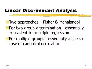
We shall now use Fisher’s linear discriminant function to derive a classification rule for assigning skulls to one of the two predefined groups on the basis of the five measurements available. Discriminant Analysis

Now proceed to complete the analysis. Discriminant Analysis

As before use the secondary screens to select the grouping variable (place) and use Define Range. Discriminant Analysis

Select the independents, use OK to run. Discriminant Analysis

From the statistics button select Discriminant Analysis Now proceed to complete the analysis.

The resulting descriptive output displays, means and standard deviations of each of the five measurements for each type of skull and overall are given in the Group Statistics table. Discriminant Analysis

The within-group covariance matrices shown in the Covariance Matrices table suggest that the sample values differ to some extent, see Box’s test for equality of covariances (see Log Determinants and Test Results). Discriminant Analysis

The within-group covariance matrices shown in the Covariance Matrices table suggest that the sample values differ to some extent, but according to Box’s test for equality of covariances (tables Log Determinants and Test Results) these differences are not statistically significant (F(15,3490) = 1.2, p = 0.25). Discriminant Analysis

It appears that the equality of covariance matrices assumption needed for Fisher’s linear discriminant approach to be strictly correct is valid here. In practice, Box’s test is not of great use since even if it suggests a departure for the equality hypothesis, the linear discriminant may still be preferable over a quadratic function. Here we shall simply assume normality for our data relying on the robustness of Fisher’s approach to deal with any minor departure from the assumption. Discriminant Analysis

The resulting discriminant analysis shows the eigenvalue (here 0.93) represents the ratio of the between-group sums of squares to the within-group sum of squares of the discriminant scores. It is this criterion that is maximized in discriminant function analysis. Discriminant Analysis

The canonical correlation is simply the Pearson correlation between the discriminant function scores and group membership coded as 0 and 1. For the skull data, the canonical correlation value is 0.694 so that 0.694 × 100 = 48% of the variance in the discriminant function scores can be explained by group differences. Discriminant Analysis

The Wilk’s Lambda provides a test for assessing the null hypothesis that in the population the vectors of means of the five measurements are the same in the two groups. The lambda coefficient is defined as the proportion of the total variance in the discriminant scores not explained by differences among the groups, here 51.8%. The formal test confirms that the sets of five mean skull measurements differ significantly between the two sites ( (5) = 18.1, p = 0.003). If the equality of mean vectors hypothesis had been accepted, there would be little point in carrying out a linear discriminant function analysis. Discriminant Analysis

Next we come to the Classification Function Coefficients. This table is displayed as a result of checking Fisher’s in the Statistics sub-dialogue box. Discriminant Analysis

Discriminant Analysis It can be used to find Fisher’s linear discrimimant function as defined by simply subtracting the coefficients given for each variable in each group giving the following result: Z = 0 09 meas1 + 0.156 meas2+ 0.005 meas3 - 0 177.meas4 - 0 177.meas5

Z = 0 09 meas1 + 0.156 meas2+ 0.005 meas3 - 0 177.meas4 - 0 177.meas5 The difference between the constant coefficients provides the sample mean of the discriminant function scores Discriminant Analysis

The coefficients defining Fisher’s linear discriminant function in the equation are proportional to the unstandardised coefficients given in the “Canonical Discriminant Function Coefficients” table which is produced when Unstandardised is checked in the Statistics sub-dialogue box. Discriminant Analysis

These scores can be compared with the average of their group means (shown in the Functions at Group Centroids table) to allocate skulls into groups. Here the threshold against which a skull’s discriminant score is evaluated is 0 0585= ½ (0 877 + 0 994) Discriminant Analysis Thus new skulls with discriminant scores above 0.0585 would be assigned to the Lhasa site (type B); otherwise, they would be classified as type A.

When variables are measured on different scales, the magnitude of an unstandardised coefficient provides little indication of the relative contribution of the variable to the overall discrimination. The “Standardized Canonical Discriminant Function Coefficients” listed attempt to overcome this problem by rescaling of the variables to unit standard deviation. Discriminant Analysis

For our data, such standardisation is not necessary since all skull measurements were in millimetres. Standardization should, however, not matter much since the within-group standard deviations were similar across different skull measures. According to the standardized coefficients, skull height (meas3) seems to contribute little to discriminating between the two types of skulls. Discriminant Analysis

A question of some importance about a discriminant function is: how well does it perform? One possible method of evaluating performance is to apply the derived classification rule to the data set and calculate the misclassification rate. Discriminant Analysis

Repeat using the following classification. Discriminant Analysis Now proceed to complete the analysis.

This is known as the re-substitution estimate and the corresponding results are shown in the Original part of the Classification Results table. According to this estimate, 81.3% of skulls can be correctly classified as type A or type B on the basis of the discriminant rule. Discriminant Analysis

However, estimating misclassification rates in this way is known to be overly optimistic and several alternatives for estimating misclassification rates in discriminant analysis have been suggested. One of the most commonly used of these alternatives is the so called leaving one out method, in which the discriminant function is first derived from only n – 1 sample members, and then used to classify the observation left out. The procedure is repeated n times, each time omitting a different observation. Discriminant Analysis

The Cross-validated part of the Classification Results table shows the results from applying this procedure. The correct classification rate now drops to 65.6%, a considerably lower success rate than suggested by the simple re-substitution rule. Discriminant Analysis

We now turn to applying cluster analysis to the skull data. Here the prior classification of the skulls will be ignored and the data simply “explored” to see if there is any evidence of interesting “natural” groupings of the skulls and if there is, whether these groups correspond in anyway with Morant’s classification. Here we will use two hierarchical agglomerative clustering procedures, complete and average linkage clustering and then k-means clustering. Discriminant Analysis

Select Analyze > Classify > Hierarchical Cluster Discriminant Analysis

In the usual way select the variables of interest Discriminant Analysis

Select the plots desired Discriminant Analysis

Select the desired method Discriminant Analysis Now proceed to complete the analysis.

The complete linkage clustering output shows which skulls or clusters are combined at each stage of the cluster procedure. First, skull 8 is joined with skull 13 since the Euclidean distance between these two skulls is smaller than the distance between any other pair of skulls. The distance is shown in the column labelled “Coefficients”. Discriminant Analysis

Second, skull 15 is joined with skull 17 and so on. Discriminant Analysis

The dendrogram is simpler to interpret. Discriminant Analysis

The dendrogram may, on occasions, also be useful in deciding the number of clusters in a data set with a sudden increase in the size of the difference in adjacent steps taken as an informal indication of the appropriate number of clusters to consider. For the dendrogram, a fairly large jump occurs between stages 29 and 30 (indicating a three- group solution) and an even bigger one between this penultimate and the ultimate fusion of groups (a two-group solution). Discriminant Analysis

For an alternate approach use Discriminant Analysis Now proceed to produce the plot

The initial steps agree with the complete linkage solution, but eventually the trees diverge with the average linkage dendrogram successively adding small clusters to one increasingly large cluster. For the average linkage dendrogram it is not clear where to cut the dendrogram to give a specific number of groups. Discriminant Analysis

Discriminant Analysis