Linear Discriminant Analysis
90 likes | 354 Vues
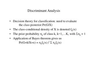
Linear Discriminant Analysis. Two approaches – Fisher & Mahalanobi For two-group discrimination - essentially equivalent to multiple regression For multiple groups - essentially a special case of canonical correlation. Based on the idea of a discriminant score

Linear Discriminant Analysis
E N D
Presentation Transcript
Linear Discriminant Analysis • Two approaches – Fisher & Mahalanobi • For two-group discrimination - essentially equivalent to multiple regression • For multiple groups - essentially a special case of canonical correlation
Based on the idea of a discriminant score Linear combination of the variables which would produce the maximally different scores across the groups LDA – Fisher’s Approach
For two group - Uses the idea of finding the locus of points equidistant from the group means For # groups > 2 We find the distance to each group centroid and assign each point to the closest centroid LDA – Mahalanobi’s Approach
Using Proc Discrim from SAS ProcDISCRIM data=iris_train out=iris_out_dis testdata=iris_test distance manova ncan=2 ; title 'Discriminant Analysis - IRIS data set'; class species; var sepallen sepalwid petallen petalwid; run; Hite rate = .9467 Error Rate = .0533 With Different training set Hit rate = 1. Discriminant Analysis - IRIS data set 30 07:58 Sunday, November 28, 2004 The DISCRIM Procedure Classification Summary for Test Data: WORK.IRIS_TEST Classification Summary using Linear Discriminant Function Generalized Squared Distance Function 2 _ -1 _ D (X) = (X-X )' COV (X-X ) j j j Posterior Probability of Membership in Each species 2 2 Pr(j|X) = exp(-.5 D (X)) / SUM exp(-.5 D (X)) j k k Number of Observations and Percent Classified into species From species SETOSA VERSICOLOR VIRGINICA Total SETOSA 24 0 0 24 100.00 0.00 0.00 100.00 VERSICOLOR 0 23 2 25 0.00 92.00 8.00 100.00 VIRGINICA 0 2 24 26 0.00 7.69 92.31 100.00 Total 24 25 26 75 32.00 33.33 34.67 100.00 Priors 0.33333 0.33333 0.33333 LDA – Iris Data set
train <- sample(1:7129, 100) z<-lda(fmat.train[,train],fy) z.predict.test<-predict(z,fmat.test[,1:3000])$class table(fy2,z.predict.test) 30 of first 60 genes fy2 ALL AML ALL 16 4 AML 10 4 Hit rate = .5882 First 60 genes fy2 ALL AML ALL 15 5 AML 6 8 Hit rate = .6765 30 of all 7129 genes fy2 ALL AML ALL 14 6 AML 3 11 Hit rate = .7353 30 of all 7129 genes fy2 ALL AML ALL 12 8 AML 8 6 Hit Rate = .5294 100 of all 7129 Genes fy2 ALL AML ALL 17 3 AML 5 9 Hit rate = .8235 First 3000 Genes fy2 ALL AML ALL 20 0 AML 9 5 Hit rate = .7353 LDA – Microarray Data
fy2 pred ALL AML ALL 20 13 AML 0 1 fy2 z.predict.test ALL AML ALL 20 9 AML 0 5 Compare LDA to SVM (1st 3000 Genes)
LDA - Goodness of fit Proportional Chance Criterion (PPC) • T-test where t=(observed hits-expected hits)/√(n*h*(1-h)) [h=hit rate associated with the PPC] • Expected # of hits = n(prob 1st group)^2+n(1-prob first group)^2 • For the microarray example • Expected # of hits = 17.52899 (.5156 hit rate) • T= 2.5637 • Gives us a P-value close to .0075 • LDA looks do a sufficient job
LDA- Problems • R was nice enough to give me this warning when # of variables was over 36 Warning message: variables are collinear in: lda.default(x, grouping, ...)