Linear Discriminant Functions in Visual Recognition
Learn about linear discriminant functions in visual recognition, their implementation in decision surfaces, and extension to multicategory cases. Explore how linear machines classify data and how generalized functions enhance discrimination abilities.

Linear Discriminant Functions in Visual Recognition
E N D
Presentation Transcript
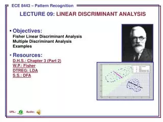
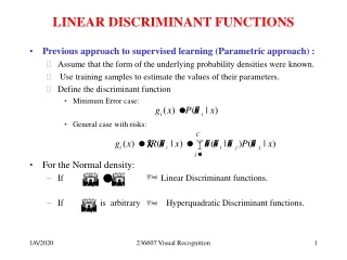
LINEAR DISCRIMINANT FUNCTIONS • Previous approach to supervised learning (Parametric approach) : • Assume that the form of the underlying probability densities were known. • Use training samples to estimate the values of their parameters. • Define the discriminant function • Minimum Error case: • General case with risks: • For the Normal density: • If Linear Discriminant functions. • If is arbitrary Hyperquadratic Discriminant functions. 236607 Visual Recognition
LINEAR DISCRIMINANT FUNCTIONS cont. • In this lecture we assume that we know the proper form of the discriminant functions, and use the samples to estimate the parameters. This approach does not require knowledge of the forms of underlying pdf's. • We will consider only linear discriminant functions. Linear discriminant functions are relatively easy to compute. 236607 Visual Recognition
LINEAR DISCRIMINANT FUNCTIONS AND DECISION SURFACESThe 2-Category Case • A linear discriminant function can be written as where w = weight vector, w0= bias or threshold ( in the next lectures we shall call it b to be close to SVM terminology) • A 2-class linear classifier implements the following decision rule: Decide w1 if g(x)>0 and w2 if g(x)<0. 236607 Visual Recognition
The 2-Category Case cont. A simple linear classifier: The equation g(x) = 0 defines the decision surface that separates points assigned to w1 from points assigned to w2. When g(x) is linear, this decision surface is a Hyperplane (H). 236607 Visual Recognition
The 2-Category Case cont. • H divides the feature space into 2 half spaces: R1 for w1, and R2 for w2. • If x1 and x2 are both on the decision surface w is normal to any vector lying in the hyperplane 236607 Visual Recognition
The 2-Category Case cont. 236607 Visual Recognition
The 2-Category Case cont. • If we express x as where xp is the normal projection of x onto H, and r is the algebraic distance from x to the hyperplane. Since g(xp)=0, we have or • r is signed distance: r > 0 if x falls in R1 , r < 0 if x falls in R2 . • Distance from the origin to the hyperplane is w0/||w|| . 236607 Visual Recognition
The Multicategory Case • 2 approaches to extend the linear discriminant functions approach to the multicategory case: • Reduce the problem to C-1 two-class problems: Problem # i: Find the functions that separates points assigned to w i from those not assigned to w i. 2. Find the c(c-1)/2 linear discriminants, one for every pair of classes • Both approaches can lead to regions in which the classification is undefined ( see the Figure ). 236607 Visual Recognition
The Multicategory Case dichotomy dichotomy 236607 Visual Recognition
The 2-Category Case cont. • Define c linear discriminant functions: • Classifier: in case of equal scores, the classification is left undefined. • The resulting classifier is called a Linear Machine. • A linear machine divides the feature space into c decision regions, with gi(x) being the largest discriminant if x is in region Ri. • If Riand Rj are contiguous, the boundary between them is a portion of the hyperplane Hij defined by: 236607 Visual Recognition
The 2-Category Case cont. • It follows that is normal to Hij • The signed distance from x to Hij is given by: • There are c(c-1)/2 pairs of regions. They are convex . • Not all regions in real life are contiguous, and the total number of hyperplane segments appearing in the decision surfaces is often fewer than c(c-1)/2. Decision boundaries: 3-class problem 5-class problem 236607 Visual Recognition
GENERALIZED LINEAR DISCRIMINANT FUNCTIONS • The linear discriminant function g(x) can be written as • By adding d(d+1)/2 additional terms involving the products of pairs of components of x, we obtain the quadratic discriminant function • The separating surface defined by g(x)=0 is a second-degree or hyperquadric surface. • By continuing to add terms such as we can obtain the class of polynomial discriminant functions. 236607 Visual Recognition
GENERALIZED LINEAR DISCRIMINANT FUNCTIONS • Polynomial functions can be thought of as truncated series expansions of some arbitrary g(x). • The generalized linear discriminant function is defined as where is a -dimensional weight vector, and is an arbitrary function of x. • The resulting discriminant function is not linear in x, but it is linear in y. • The functions map points in d -dimensional x-space to points in -dimensional y-space. 236607 Visual Recognition
Example1 • Let the quadratic discriminant function be The 3-dimensional vector y is then given by 236607 Visual Recognition
Example2. • Whenever is degenerate. • The plane H defined by divides the y-space into 2 decision regions R1 and R2. • If • Decision regions in the original x-space: 236607 Visual Recognition
THE TWO-CATEGORY LINEARLY-SEPARABLE CASE where x0=1. • Let - augmented feature vector (trivial mapping from d-dimensional x-space to (d+1)-dimensional y-space) and augmented weight vector. Then . The hyperplane decision surface defined passes through the origin in y-space. The distance from any point y to is given by , or Because this distance is less then distance from x to H. The problem of finding [w0,w] is changed to a problem of finding vector 236607 Visual Recognition
THE TWO-CATEGORY LINEARLY-SEPARABLE CASE • Suppose that we have a set of n samples some labeled w1 and some labeled w2. • Use these training samples to determine the weights . • Look for a weight vector that classifies all the samples correctly. • If such a weight vector exists, the samples are said to be linearly separable. A sample yi is classified correctly if or 236607 Visual Recognition
THE TWO-CATEGORY LINEARLY-SEPARABLE CASE • If we replace all the samples labeled w2 by their negatives, then we can look for a weight vector such that for all the samples. Such a weight vector is called a separating vector or more generally a solution vector. • Each sample places a constraint on the possible location of a solution vector. • defines a hyperplane through the origin having as a normal vector. • The solution vector (if it exists) must be on the positive side of every hyperplane • Intersection of the n half-spaces = Solution Region 236607 Visual Recognition
THE TWO-CATEGORY LINEARLY-SEPARABLE CASE • Any vector that lies in the solution region is a solution vector. • The solution vector (if it exists) is not unique. • We can impose additional requirements to find a solution vector closer to the middle of the region (the resulting solution is more likely to classify new test samples correctly). 236607 Visual Recognition
THE TWO-CATEGORY LINEARLY-SEPARABLE CASE • Seek a unit-length weight vector that maximizes the minimum distance from the samples to the separating plane. • Seek the minimum-length weight vector satisfying • The solution region shrinks by margins b/||yi|| The new solution lies within the previous region 236607 Visual Recognition
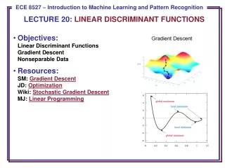
GRADIENT DESCENT PROCEDURES • Define a criterion function that is minimized if is a solution vector ( for all samples). • Start with some arbitrarily chosen weight vector . • Compute the gradient vector . • The next value is obtained by moving a distance from in the direction of steepest descent (i.e. along the negative of the gradient) . • In general, is obtained from using where is learning rate. 236607 Visual Recognition
GRADIENT DESCENT algorithm begininitialize do until return end • How to set the learning rate ? Suppose 236607 Visual Recognition
GRADIENT DESCENT algorithm where is the Hessian matrix evaluated at Substituting into (2) from (1) By equating to zero a derivative with respect to we get: 236607 Visual Recognition
Newton’s algorithm. Choose a(k+1) to minimize (2) : equate to zero a derivative of the r.h.s. of (2) with respect to a and then substitute a(k+1) in place of a 236607 Visual Recognition
Newton’s algorithm. begininitialize do until return end • Newton’s algorithm gives a greater improvement per step, then gradient descent, but is not applicable , when Hessian is singular and also takes O(d3) time. 236607 Visual Recognition
MINIMIZING THE PERCEPTRON CRITERION FUNCTION • Perceptron criterion function: is the set of samples misclassified by . • If no samples are misclassified, is empty, and • Since if is misclassified, is never negative, and is zero only if is a solution vector. • Geometrically, is proportional to the sum of the distances from the misclassified samples to the decision boundary. • Since the update rule becomes where is the set of samples misclassified by . 236607 Visual Recognition
TheBatch Perceptron Algorithm begininitialize do until return end 236607 Visual Recognition
Perceptron Algorithm cont. Sequence of misclassified samples: y2,y3,y1,y3 236607 Visual Recognition
TheFixed-Increment Single-Sample Perceptron begininitialize do until all patterns properly classified return a end 236607 Visual Recognition
Perceptron Algorithm - Comments • The perceptron algorithm adjusts the parameters only when it encounters an error, i.e. misclassified training example . • Correctly classified examples can be ignored. • The learning rate can be chosen arbitrary, it will only impact on the norm of the final vector w (and the corresponding magnitude of w0). • The final weight vector is a linear combination of training points 236607 Visual Recognition
RELAXATION PROCEDURES • Another criterion function that is minimized when is a solution vector: where still denotes the set of training samples misclassified by . • The advantages of Jq over Jp is that its gradient is continuous, whereas the gradient of Jp is not. Jq presents a smoother surface to search. • Disadvantages: • Jq is so smooth near the boundary of the solution region that the sequence of weight vectors can converge to a point on the boundary a=0 • The value of Jq can be dominated by the longest sample vectors. 236607 Visual Recognition
RELAXATION PROCEDURES cont. • Solution of these problems: • Use the following criterion function: where denotes the set of samples for which • If is empty, define . • Jr is never negative . • Jr =0 if and only if for all the training samples. • The gradient of Jr is given by 236607 Visual Recognition
RELAXATION PROCEDURES cont. • Update rule for batch relaxation with margin: 236607 Visual Recognition
Nonseparable Behavior • The Perceptron and Relaxation procedures are methods for finding a separating vector when the samples are linearly separable. They are error correcting procedures. • Even if a separating vector is found for the training samples, it does not follow that the resulting classifier will perform well on independent test data. • To ensure that the performance on training and test data will be similar, many training samples should be used. • Unfortunately, sufficiently large training samples are almost certainly not linearly separable. • No weight vector can correctly classify every sample in a nonseparable set 236607 Visual Recognition
Nonseparable Behavior • The corrections in the Perceptron and Relaxation procedures can never cease. If set is nonseparable. • If we choose then we can get acceptable performance on nonseparable problems while preserving the ability to find a separating vector on separable problems. • The rate at which approaches zero is important: • Too slow: Results will be sensitive to those training samples that render the set nonseparable. • Too fast Weight vector may converge prematurely with less than optimal results. • We can make a function of recent performance, decreasing it as performance improves. • We can choose 236607 Visual Recognition
MINIMUM SQUARED ERROR PROCEDURES • The MSE approach sacrifices the ability to obtain a separating vector for good compromise performance on both separable and nonseparable problems. • The Perceptron and Relaxation procedures use the misclassified samples only. • Previously, we sought a weight vector making all of the inner products • In the MSE procedure, we will try to make , where bi are some arbitrarily specified positive constants. • Using matrix notation: 236607 Visual Recognition
MINIMUM SQUARED ERROR PROCEDURES cont. • Using matrix notation: or • If Y is nonsingular, then • Unfortunately, Y is not a square matrix, usually with more rows than columns. 236607 Visual Recognition
MINIMUM SQUARED ERROR PROCEDURES cont. • When there are more equations than unknowns, is overdetermined, and ordinarily no exact solution exists. • We can seek a weight vector that minimizes some function of an error vector e • Minimize the squared length of the error vector, which is equivalent to minimizing the sum-of-squared-error criterion function • Setting the gradient equal to zero, we get the following necessary condition 236607 Visual Recognition
MINIMUM SQUARED ERROR PROCEDURES cont. • is a square matrix, and often nonsingular. Therefore, we can solve for using 236607 Visual Recognition
MINIMUM SQUARED ERROR PROCEDURES cont. where is called pseudoinverse of Y. is defined more generally by It can be shown that this limit always exists is MSE solution to • Different choices of b give the solution different properties. 236607 Visual Recognition
Example Suppose we have the following two-dimensional points for the two categories: w1: and , and w2 : and Four training points and decision boundary 4 R2 3 2 1 R1 1 2 3 4v 0 236607 Visual Recognition
Example Our matrix Y is Pseudoinverse is If arbitrarily let all the margins be equal: we shall find the solution 236607 Visual Recognition
Relation to Fisher’s Linear Discriminant • With special choice of the vector b, the MSE is connected to Fisher’s linear discriminant. Assume nd-dimensional samples n1 are from D1 and n2 are from D2 The matrix Y can be written: where 1i is a column vector of ni ones, and Xi is an ni-by-d matrix which rows are labeled wi. We partition a and b : 236607 Visual Recognition
Relation to Fisher’s Linear Discriminant cont. • Let’s write • Remember that sample mean is and 236607 Visual Recognition
Relation to Fisher’s Linear Discriminant cont. • We can multiply matrices in (4): • From the first row we have and from the second 236607 Visual Recognition
Relation to Fisher’s Linear Discriminant cont. • But the vector is in the direction of for any value of , thus we can write for some scalar a . • Then (10) yields which is proportional to the Fisher linear discriminant. The decision rule is decide otherwise decide 236607 Visual Recognition
THE WIDROW-HOFF PROCEDURE • The criterion function could be minimized by a gradient descent procedure. • Advantages: • Avoids the problems that arise when is singular. • Avoids the need for working with large matrices. • Since a simple update rule would be If we consider the samples sequentially 236607 Visual Recognition
THE WIDROW-HOFF PROCEDURE • Widrow-Hoff or LMS (Least-Mean-Square) procedure • Initialize do until return end 236607 Visual Recognition