Linear Discriminant Functions Chapter 5 (Duda et al.)

1. Linear Discriminant FunctionsChapter 5 (Duda et al.) CS479/679 Pattern RecognitionDr. George Bebis

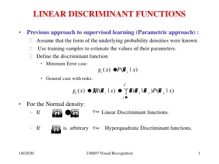
2. Discriminant Functions:two-categories case • Decide w1 if g(x) > 0 and w2 if g(x) < 0 • If g(x)=0, then x lies on the decision boundary and can be assigned to either class. • Classification is viewed as findinga decision boundarythat separates the data belonging to different classes.

3. Statistical vs Discriminant Approach • Statistical approaches find the decision boundary by first estimating the probability distribution of the patterns belonging to each class. • Discriminant approaches find the decision boundary explicitly without assuming a probability distribution.

4. Discriminant Approach • Specify parametric form of the decision boundary (e.g., linear or quadratic). • Find the best decision boundary of the specified form using a set of training examples xk. • This is performed by minimizing a criterion function (e.g., “training error” or “sample risk”): correct class predicted class

5. Linear Discriminant Functions:two-categories case • A linear discriminant function has the following form: • The decision boundary, given byg(x)=0, is a hyperplane where the orientation of the hyperplane is determined by w and its location by w0. • w is the normal to the hyperplane • If w0=0, the hyperplane passes through the origin

6. Geometric Interpretation of g(x) • g(x) provides an algebraic measure of the distance of x from the hyperplane. x can be expressed as follows: direction of r

7. Geometric Interpretation of g(x) (cont’d) • Substitute the previous expression in g(x): since and

8. Geometric Interpretation of g(x) (cont’d) • Therefore, the distance of x from the hyperplane is given by: setting x=0:

9. Linear Discriminant Functions: multi-category case • There are several ways to devise multi-category classifiers using linear discriminant functions: (1) One against the rest (i.e., c-1 two-class problems) problem: ambiguous regions

10. Linear Discriminant Functions: multi-category case (cont’d) (2) One against another (i.e., c(c-1)/2 pairs of classes) problem: ambiguous regions

11. Linear Discriminant Functions: multi-category case (cont’d) • To avoid the problem of ambiguous regions: • Define c linear discriminant functions • Assign x to wi if gi(x) > gj(x) for all j  i. • The resulting classifier is called a linear machine (see Chapter 2 too)

12. Linear Discriminant Functions: multi-category case (cont’d) • A linear machine divides the feature space in c convex decisions regions. • If x is in region Ri, the gi(x) is the largest. c(c-1)/2 pairs of regions but typically less decision boundaries

13. Linear Discriminant Functions: multi-category case (cont’d) • The boundary between two regions Ri and Rj is a portion of the hyperplane Hij given by: • (wi-wj) is normal to Hij and the signed distance from x to Hij is

14. Higher Order Discriminant Functions • Can produce more complicated decision boundaries than linear discriminant functions. Linear discriminant: hyperquadric decision boundaries

15. Generalized discriminants - α is a dimensional weight vector - the functions yi(x) are called φ functions • yi(x) map points from the d-dimensional x-space to the -dimensional y-space (usually >> d )

16. Generalized discriminants • The resulting discriminant function is not linear in x but it is linear in y. • The generalized discriminant separates points in the transformed space by a hyperplane passing through the origin.

17. Example d=1, • The corresponding decision regions R1,R2in the x-space are not simply connected! φ functions

18. Example (cont’d) g(x) maps a line in x-space to a parabola in y-space. The plane αty=0 divides the y-space in two decision regions

19. Learning: two-category, linearly separable case • Given a linear discriminant function the goal is to learn the parameters w and w0 using a set of n labeled samples xiwhere each xi has a class label ω1 or ω2.

20. Simplified notation: augmented feature/weight vectors dimensionality: d  (d+1)

21. Classification in augmented space Classification rule: If αtyi>0 assign yi to ω1 else if αtyi<0 assign yi to ω2 g(x)=αty Discriminant:

22. Learning: two-category, linearly separable case • Given a linear discriminant function the goal is to learn the weights (parameters) α using a set of n labeled samples yi where each yi has a class label ω1 or ω2. g(x)=αty

23. Effect of training examples on solution • Every training sample yi places a constraint on the weight vector α. • αty=0 defines a hyperplane in parameter space having y as a normal vector. • Given n examples, the solution α must lie on the intersection of n half-spaces. a2 g(x)=αty parameter space (ɑ1, ɑ2) a1

24. Effect of training examples on solution (cont’d) Solution can be visualized either in the parameteror featurespace. parameter space (ɑ1, ɑ2) feature space (y1, y2) a2 a1

25. Solution Uniqueness/Constraints Solution vector is usually not unique; we can impose certain constraints to enforce uniqueness, e.g.,: Example 1: Find unit-length weight vector that maximizes the minimum distance from the samples to the separating plane.

26. Solution Uniqueness/Constraints (cont’d) Example 2: Find minimum-length weight vector satisfying the constraint shown below where b is a positive constant called margin.

27. Learning: two-category linearly separable case (cont’d) parameter space (ɑ1, ɑ2) Key objective is to move solution to the center of the feasible regionas this solution is more likely to classify new test samples correctly.

28. Normalized Version Ifyiin ω2, replace yi by -yi Find α such that: αtyi>0 replace yi by -yi

29. Iterative Optimization • Define an error function J(α) (e.g., based on training samples) that is minimized if α is a solution vector. • Minimize J(α) iteratively: search direction α(k) α(k+1) learning rate

30. Gradient Descent Method learning rate aα

31. Gradient Descent (cont’d) solution space ɑ

32. Gradient Descent (cont’d) • What is the effect of the learning rate? η η slow but converges to solution fast by overshoots solution

33. Gradient Descent (cont’d) • How to choose the learning rate h(k)? • If J(α) is quadratic, then H is constant which implies that the learning rate is constant! Taylor series approximation Hessian (2nd derivatives) optimum learning rate

34. Newton’s Method requires inverting H aα

35. Newton’s method (cont’d) If J(α) is quadratic, Newton’s method converges in one step!

36. Gradient descent vs Newton’s method

37. Perceptron rule • Apply Gradient Descent Rule assuming: where Y(α) is the set of samples misclassified by α. • If Y(α) is empty, Jp(α)=0; otherwise, Jp(α)>0 (normalized version)

38. Perceptron rule (cont’d) • The gradient of Jp(α) is: • The perceptron update rule is obtained using gradient descent: aα or

39. Perceptron rule (cont’d) aα YkY(α) all missclassified examples

40. Perceptron rule (cont’d) • Move the hyperplane so that training samples are on its positive side. a2 a2 Example 1 Example 2 a1 a1

41. Perceptron rule (cont’d) η(k)=1 one example at a time Perceptron Convergence Theorem: If training samples are linearly separable, then the sequence of weight vectors by the above algorithm will terminate at a solution vector in a finite number of steps.

42. Perceptron rule (cont’d) order of examples: y2 y3 y1 y3

43. Perceptron rule (cont’d) • Generalizations: Variable learning rate and a margin

44. Perceptron rule (cont’d)

45. Perceptron rule (cont’d)

46. Relaxation Procedures • Note that different criterion functions exist • One possible choice is: • Where Y is again the set of the training samples that are misclassified by a • However, there are two problems with this criterion • The function is too smooth and can converge to a=0 • Jq is dominated by training samples with large magnitude

47. Relaxation Procedures (cont’d) • A modified version that avoids the above two problems is • Here Y is the set of samples for which its gradient is given by:

48. Relaxation Procedures (cont’d)

49. Relaxation Procedures (cont’d)

50. Relaxation Procedures (cont’d)