Linear Discriminant Analysis (LDA) for selection cuts :
390 likes | 582 Vues
Julien Faivre. Alice week Utrecht – 14 June 2005. Linear Discriminant Analysis (LDA) for selection cuts :. Motivations Why LDA ? How does it work ? Concrete examples Conclusions and S.Antonio’s present. Observables : Production yields Spectra slope

Linear Discriminant Analysis (LDA) for selection cuts :
E N D
Presentation Transcript
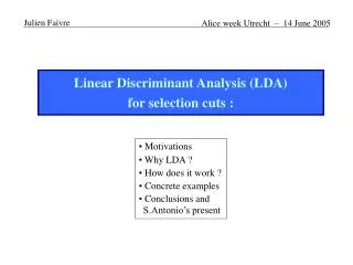
Julien Faivre Alice week Utrecht – 14 June 2005 Linear Discriminant Analysis (LDA)for selection cuts : • Motivations • Why LDA ? • How does it work ? • Concrete examples • Conclusions andS.Antonio’s present
Observables : • Production yields • Spectra slope • p, azimutal anisotropy (v2) • Scaled spectra (RCP, RAA), v2 • Statistics is needed for : • p-p collisions, low-p • All p • All p • Peripheral, p-p, high-p • Need more statistics • Need fast and easy selection optimization Apply a patternclassification method 1/15 Julien Faivre Alice week Utrecht – 14 Jun 2005 Initial motivations : Some particles are critical at all p and in all collision systems • Examples of initial S/N ratios : • @RHIC = 10-10@RHIC = 10-11D0@LHC = 10-8
b b a a Variable 1 Variable 1 2/15 Julien Faivre Alice week Utrecht – 14 Jun 2005 Basic strategy : the « classical cuts » • Want to extract signal out of background • « Classical cuts » : example with n = 2 variables (actual analysis : 5-to 30+) • For a good efficiency on signal (recognition), pollution by background ishigh (false alarms) • Compromise has to be found between good efficiency and high S/N ratio • Tuning the cuts is long and difficult Variable 2 Variable 2
3/15 Julien Faivre Alice week Utrecht – 14 Jun 2005 Which pattern classification method ? • Bayesian decision theory • Markov fields, hidden Markov models • Nearest neighbours • Parzen windows • Linear Discriminant Analysis • Neural networks • Unsupervised learning methods Linear Discriminant Analysis (LDA) Neural networks • Linear • Simple training • Simple tuning Fast tuning • Linear shapeBut multicut OK • Connex shape • Non linear • Complex training Overtraining • Choose layers & neurons Long tuning • Non linear shape • Non connex shape • Only advantage of neural nets choose LDA Not an absolute answer ;just tried and turns out it works fine
Variable 2 Best axis Variable 1 4/15 Julien Faivre Alice week Utrecht – 14 Jun 2005 LDA mechanism : • Simplest idea : cut along linear combination of the n observables := LDA axis Cut on scalar product
Need a criterium to find the LDA direction • Direction found will depend on the criterium chosen • Fisher criterium (widely used) : • Projection of the points on direction gives distributions of classes 1 and 2along this direction • i = mean of distrib. i • i = width of distrib. i • 1 and 2 have to be as far as possible one from the other, 1 and 2 have to be as small as possible 2- 1 1 2 1 2 5/15 Julien Faivre Alice week Utrecht – 14 Jun 2005 LDA criterium : Fisher : LDA axis
6/15 Julien Faivre Alice week Utrecht – 14 Jun 2005 Improvements needed : • Fisher-LDA doesn’t work for us : • too much background, too few signal ; • background covers all the area where signal lies • Fisher-LDA « considers » the distributions as gaussian(mean and width) insensitive to local parts of the distributions Fisher good (not us) Fisher not good (us) (log) • Solutions : • Apply several successive LDA cuts • Change the criterium : Fisher « optimized »
Variable 2 Variable 1 1st best axis • Criterium « optimized I » : Given an efficiency of the kth LDA-cut on the signal, maximisation of the number of background cut 2nd best axis 7/15 Julien Faivre Alice week Utrecht – 14 Jun 2005 Multi-cut LDA & optimized criterium : • Fisher is global irrelevant for multi-cut LDA • Have to find criterium thatdepends locally on thedistributions, not globally • More cuts = better description of the « signal/background boundary » • BUT : if many cuts, tends to describe too locally
8/15 Julien Faivre Alice week Utrecht – 14 Jun 2005 Non-linear approaches : Caution with the description of the boundary : Too local description bad performance Over training sample : Over test sample : Straight line : mmmh… Not so bad Curve : still not satisfied Very good Almost candidate-per-candidate : happy Very bad Case of LDA : the more cuts, the better the limit is known(determined from number of background candidates cut) everything under control !
Classical cuts Gain Minimal relative uncertaintywith LDA 28th LDA dir. 29th LDA direction 31st LDA direction 30th LDA direction 9/15 Julien Faivre Alice week Utrecht – 14 Jun 2005 LDA cut-tuning : LDA tightening Best LDA cut value
10/15 Julien Faivre Alice week Utrecht – 14 Jun 2005 LDA for STAR’s hyperons : • Jeff Speltz’s 62 GeV K (topological) analysis (SQM 2004) : Classical LDA + 63 % signal
11/15 Julien Faivre Alice week Utrecht – 14 Jun 2005 LDA in ALICE : • Ludovic Gaudichet : strange particles (topologically) K, , then and - Neural nets don’t even reach optimized classical - Cascaded neural nets do but don’t do better - LDA seems to do better (ongoing study) • J.F. : charmed meson D0 in K (topologically) - Very preliminary results on p-integrated raw yield (PbPb central) : (« Current classical cuts » : Andrea Dainese’s thesis, PPR) - Statistical relative uncertainty (S/S) on PID-filtered candidates : Current classical = 4.4%LDA = 2.1% 2.1 times better - Statistical relative uncertainty on “unfiltered” cand. (just (,)’s out) : Current classical = 4.3%LDA = 1.6% 2.7 times better - Looking at LDA distributions new classical set found : Does 1.6 times better than current classical
11bis/15 Julien Faivre Alice week Utrecht – 14 Jun 2005 LDA in ALICE (comparison) : VERY PRELIMINARY !! Optimized classical LDA
Significance vs signal Purity-efficiency plot Optimal LDA cut(tuned wrt relative uncertainty) LDA cuts Current classical cuts New classical cuts 12/15 Julien Faivre Alice week Utrecht – 14 Jun 2005 LDA in ALICE (performance) : PID-filtered D0’s with quite tight classical pre-cuts applied
Zoom 13/15 Julien Faivre Alice week Utrecht – 14 Jun 2005 LDA in ALICE (tuning) : • Tuning = search of the minimum of a valley-shaped 1-dim function • 2 hypothesis of background estimation Relative uncertainty vs efficiency LDA Current classical New classical Optimal LDA
Performance : better than classical cuts • Cut-tuning : obvious (classical cuts : nightmare) cool for other centrality classes, collision energies, colliding systems, p ranges Also provides systematics : - LDA vs classical, - Changing LDA cut value, - LDA set 1 vs LDA set 2 Cherry on the cake : optimal usage of ITS for particle with long c’s (,K,,) : • 6 layers & 3 daughter tracks • 343 hit combinations / sets of classical cuts !! Add 3 variables to LDA (#hits of each daughter) automatic ITS cut-tuning 14/15 Julien Faivre Alice week Utrecht – 14 Jun 2005 Conclusion : • The method we have now : • Linear • Easy implementation (as classical cuts)and class ready ! (See next slide) • Better usage of the N-dim information • Multicut not as limited as Fisher • Provides transformation from Rn to R trivial optimization of the cuts • Know when limit (too local) is reached Strategy could be :1- tune LDA2- derive classical from LDA
15/15 Julien Faivre Alice week Utrecht – 14 Jun 2005 S. Antonio’s present : available tool : • C++ class which performs LDA is available • Calculates LDA cuts with chosen method, params and variable rescaling • Has a function Pass to check if a candidate passes the calculated cuts • Plug-and-play : whichever the analysis, no change in the code required • « Universal » input format (tables) • Ready-to-use : options have default values don’t need to worry for a 1st look • Code is documented for how to use (examples included) • Full documentation about LDA and optimization available • Example of filtering code which makes plot like in previous slide available • Not yet on the web, send e-mail (julien.faivre@pd.infn.it) • Statistics needed for training : with optimized criterium, looks like2000 S and N after cuts are enough
Another fake Xi Destroyed Fake Xi Created • Destroys signal • Keeps background • Destroys some correlations Has to be studied 19/25 IV. Rotating Rotating : Padova – 22 Febbraio 2005 Fake Xi Real Xi Nothing (GeV/c2)
2 classes : • Signal (real Xis) • Bkgnd (combinatorial) • 1 type : Xi vertex • Dca’s • Decay length • Number of hits • Etc… • Background sample : real data • Signal sample : simulation (embedding) Goal :Classify a new object in one of the classes defined Usage : Observed XiVertex = signal or background IV. Linear Discriminant Analysis Pattern classification : 1/100 Learning : • p classes of objects of the same type • n observables, defined for all the classes • p samples of Nk objects for each class k
IV. Linear Discriminant Analysis Fisher criterium : 1/100 • Fisher-criterium : maximisation of • No need to have a maximisation algorithm • LDA direction u is directly given by : • All done with simple matrices operations • Calculating axis way faster than reading data Within-class scatter matrix Mean-vectors
Julien Faivre – III. Fisher LDA Mathematically speaking (I) : Yale – 04 Nov 2003 • Fisher-criterium : maximisation of • Let’s call u the vector of the LDA axis, xk the vector of the kth candidate for the training (learning) • Means for class i (vector) : • Mean of the projection on u for class i : • So : 16/42
Julien Faivre – III. Fisher LDA Mathematically speaking (II) : Yale – 04 Nov 2003 • Now : • Let’s defineand Sw = S1 + S2 : • So : • In-one-shot booking of the matrix : 17/42
IV. Linear Discriminant Analysis Algorithm for optimized criterium : 1/100 • First find Fisher LDA direction, as a start point • Do a « performance function » : : vector u performance figure • Maximize the « performance figure » by varying the direction of u • Several methods for maximisation : • Easy and fast : one coordinate at a time • Fancy and powerfull : genetic algorithm
IV. Linear Discriminant Analysis One coordinate at a time : 1/100 • Change the direction of u by steps of a constant angle : = 8 to start, then = 4, 2, 1, eventually 0.5 • Change the 1st coordinate of u until reaches a maximum • Change all the other coordinates like this, one by one • Then, try again with 1st coordinate, and with the other ones • When no improvement anymore : divide by 2 and do the whole thing again
Julien Faivre – IV. Improvements Genetic algorithm (I) : Yale – 04 Nov 2003 • Problem with the « one-coordinate-at-a-time » algo : likely to fall in a local maximum different than the absolute maximum • So : use genetic algorithm ! • Like genetic evolution : • Pool of chromosomes • Generations : evolution, reproduction • Darwinist selection • Mutations 28/42
Julien Faivre – IV. Improvements Genetic algorithm (II) : Yale – 04 Nov 2003 • Start with p chromosomes (p vectors uk) made randomly from Fisher • Calculate performance figure of each uk • Order the p vectors by decreasing value of the performance figure • Keep only the m first vectors (Darwinist selection) • Have them make children : build a new set of p chromosomes, with the m selected ones and combinations of them • In the children chromosomes, introduce some mutations (modify randomly a coordinate) • New pool is ready : go to 29/42
IV. Linear Discriminant Analysis Statistics needed : 1/100 • Fisher-LDA : samples need to have more than 10000 candidates each • Doesn’t depend on number of observables (?) (n = 10, n = 22) • Optimized criteria : need much more • Guess : at minimum 50000 candidates per sample, maybe up to 500000 ? • Depends on number of observables
Julien Faivre – IV. Improvements Statistics needed (II) : Yale – 04 Nov 2003 • Optimised criterium : can’t look at the oscillations to know if enough statistics ! Optimised criterium (step 1) Variable 2 Variable 2 Optimised criterium(step 2) Variable 1 Variable 1 31/42
Julien Faivre – IV. Improvements Statistics needed (III) : Yale – 04 Nov 2003 • Solutions : • Try all the combinations of k out of n observables (never used) • Problem : number is huge (2n-1) : n = 5 31 combinations,n = 10 1023 combinations, n = 20 1048575 combinations ! • Use underoptimal LDA (widely used) • See next slide • Use PCA : Principal Components Analysis (widely used) • See one after next slide 32/42
Julien Faivre – V. Various things Part V – Various things : Yale – 04 Nov 2003 • The projection of the LDA direction from the n-dimension space to a k-dimension sub-space is not the LDA direction of the projection of the samples from the n-dimension space to the k-dimension sub-space • The more observables, the better • Mathematically : adding an observable can’t lower discriminancy • Practically : it can, because of limited statistics to train • LDA (multi-cuts) can’t do worse than cutting on each observable • Because cutting on each observable is a particular case of multi-cuts LDA ! • If does worse : criterium isn’t good, or efficiency of cuts not well chosen 38/42
Most discriminating pair containing most discriminating direction Actual most discriminating pair Most discriminating direction Julien Faivre – IV. Improvements Underoptimal LDA : Yale – 04 Nov 2003 • Calculate discriminancy of each of the n observables • Choose the observable that has the highest discriminancy • Calculate discriminancy of each pair of observables containing the previously found • Choose the most discriminating pair • Etc… with triplets, up to desired number of directions • Problem : 33/42
Variable 2 Variable 1 Julien Faivre – IV. Improvements PCA – Principal Components Analysis (I) : Yale – 04 Nov 2003 • Tool used in data reduction (e.g. image compression) • Read Root class description of TPrincipal • Finds along which directions (linear combinations of observables) is most of the information Primary component axis x1 Secondary component axis x2 Main information of a point is x1, dropping x2 isn’t important 34/42
Julien Faivre – IV. Improvements PCA – Principal Components Analysis (II) : Yale – 04 Nov 2003 • All is matrix-based : easy • « Informativeness » of the direction is given by normalised eigenvalues • Use with LDA : prior to finding the axis : • Observables = base B1 of the n-dimension space • Apply PCA over signal+bkgnd samples (together) : get base B2 of the the n-dimension space • Choose the k most informative directions : C2, subset of B2 • Calculate LDA axis in space defined by C2 • If several LDA directions ? No problem : apply PCA but keep all information of the candidates : just don’t use it all for LDA PCA will give different sub-space for each step 35/42
Variable 2 Variable 1 Julien Faivre – IV. Improvements PCA – Principal Components Analysis (III) : Yale – 04 Nov 2003 • Problem of using PCA prior to LDA : • Use it / not use it is purely empirical • Percentage of the eigenvalues to keep is also purely empirical Best discriminating axis PCA 1st direction 36/42
Julien Faivre – IV. Improvements PCA – Principal Components Analysis (IV) : Yale – 04 Nov 2003 • Difference between PCA and LDA : • Example with letters O and Q : • PCA finds where most of the information is : Most important part of O and Q is a big round shape applying PCA means that both O and Q become O • LDA finds where most of the difference is : Difference between O and Q is the line at the bottom-right applying LDA means finding this little line PCA vs LDA 37/42
Julien Faivre – V. Various things Influence of an LDA cut : Yale – 04 Nov 2003 • Usefull to know if LDA cuts steeply or uniformly, along each direction • fk = distribution of a sample along direction of observable k • gk = the same, after the LDA cut • F the normalised integral of f • h(x) = (g/f)(F-1(x)) • Q = 0 cut uniform, Q = 1 cut steep g/f 1 0 1 F 40/42
V0 decay topology : 40/42
