What statistical analysis should I use?
Friedman test Reshaping data Ordered logistic regression Factorial logistic regression Correlation Simple linear regression Non-parametric correlation Simple logistic regression Multiple regression Analysis of covariance Multiple logistic regression Discriminant analysis One-way MANOVA

What statistical analysis should I use?
E N D
Presentation Transcript
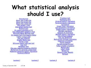
Friedman test Reshaping data Ordered logistic regression Factorial logistic regression Correlation Simple linear regression Non-parametric correlation Simple logistic regression Multiple regression Analysis of covariance Multiple logistic regression Discriminant analysis One-way MANOVA Multivariate multiple regression Canonical correlation Factor analysis Normal probability plot Tukey's ladder of powers Median split Likert Scale Winsorize General Linear Models Epilogue What statistical analysis should I use? Introduction About the A data file About the B data file About the C data file One sample t-test One sample median test Binomial test Chi-square goodness of fit Two independent samples t-test Wilcoxon-Mann-Whitney test Chi-square test (Contingency table) Fisher's exact test One-way ANOVA Kruskal Wallis test Paired t-test Wilcoxon signed rank sum test Sign test McNemar test One-way repeated measures ANOVA Bonferroni for pairwise comparisons Repeated measures logistic regression Factorial ANOVA Lecture 1Lecture 2Lecture 3Lecture 4 Tuesday, 16 September 20146:07 AM
What statistical analysis should I use? Likert Scale Linear regression - Simple linear regression Logistic regression - Simple logistic regression Logistic regression - Repeated measures logistic regression Logistic regression - Ordered logistic regression Logistics regression - Factorial logistic regression Logistic regression - Multiple logistic regression MANOVA - One-way MANOVA McNemar test Median split Median test - One sample median test Multiple regression Multiple regression - Multivariate multiple regression Normal probability plot Reshaping data Sign test t test - One sample t-test t-test - Two independent samples t-test t-test - Paired t-test Tukey's ladder of powers Wilcoxon-Mann-Whitney test Wilcoxon signed rank sum test Winsorize ANCOVA - Analysis of covariance ANOVA - One-way ANOVA ANOVA - One-way repeated measures ANOVA ANOVA - Factorial ANOVA Binomial test Bonferroni for pairwise comparisons Chi-square goodness of fit Chi-square test (Contingency table) Correlation Correlation - Non-parametric correlation Correlation - Canonical correlation Data - About the A data file Data - About the B data file Data - About the C data file Discriminant analysis Epilogue Factor analysis Fisher's exact test Friedman test General Linear Models Introduction Kruskal Wallis test 2 Tuesday, 16 September 20146:07 AM
Introduction For a useful general guide see Policy: Twenty tips for interpreting scientific claims : Nature News & CommentWilliam J. Sutherland, David Spiegelhalter and Mark Burgman Nature Volume: 503, Pages: 335–337 Date published: (21 November 2013). Some criticism has been made of their discussion of p values, see Replication, statistical consistency, and publication bias G. Francis, Journal of Mathematical Psychology, 57 (5) (2013), pp. 153–169. IndexEnd 3
Introduction These examples are loosely based on a UCLA tutorial sheet. All can be realised via the syntax window, when appropriate command strokes are also indicated . These pages show how to perform a number of statistical tests using SPSS. Each section gives a brief description of the aim of the statistical test, when it is used, an example showing the SPSS commands and SPSS (often abbreviated) output with a brief interpretation of the output. IndexEnd 4
About the A data file Most of the examples in this document will use a data file called A, high school and beyond. This data file contains 200 observations from a sample of high school students with demographic information about the students, such as their gender (female), socio-economic status (ses) and ethnic background (race). It also contains a number of scores on standardized tests, including tests of reading (read), writing (write), mathematics (math) and social studies (socst). 5
About the A data file Syntax:- display dictionary /VARIABLES id female race ses schtyp prog read write math science socst. 6
About the A data file IndexEnd 7
A one sample t-test allows us to test whether a sample mean (of a normally distributed interval variable) significantly differs from a hypothesized value. For example, using the A data file, say we wish to test whether the average writing score (write) differs significantly from 50. Test variable writing score (write), Test value 50.We can do this as shown below. Menu selection:- Analyze > Compare Means > One-Sample T test Syntax:- t-test /testval = 50 /variable = write. One sample t-test
One sample t-test Note the test value of 50 has been selected
One sample t-test The mean of the variable write for this particular sample of students is 52.775, which is statistically significantly different from the test value of 50. We would conclude that this group of students has a significantly higher mean on the writing test than 50. This is consistent with the reported confidence interval (1.45,4.10) that is (51.45,54.10) which excludes 50, of course the mid-point is the mean. IndexEnd 10
A one sample median test allows us to test whether a sample median differs significantly from a hypothesized value. We will use the same variable, write, as we did in the one sample t-test example above, but we do not need to assume that it is interval and normally distributed (we only need to assume that write is an ordinal variable). Menu selection:- Analyze > Nonparametric Tests > One Sample Syntax:- nptests /onesample test (write) wilcoxon(testvalue = 50). One sample median test
One sample median test Choose customize analysis 13
One sample median test Only retain writing score 14
One sample median test Choose tests tick “compare median…” and enter 50 as the desired value. Finally select the “run” button 15
One sample median test We would conclude that this group of students has a significantly higher median on the writing test than 50. IndexEnd 16
A one sample binomial test allows us to test whether the proportion of successes on a two-level categorical dependent variable significantly differs from a hypothesized value. For example, using the A data file, say we wish to test whether the proportion of females (female) differs significantly from 50%, i.e., from .5. We can do this as shown below. Two alternate approaches are available. Either Menu selection:- Analyze > Nonparametric Tests > One Sample Syntax:- npar tests /binomial (.5) = female. Binomial test
Binomial test Choose customize analysis 19
Binomial test Only retain female 20
Binomial test Choose tests tick “compare observed…” and under options 21
Binomial test enter .5 as the desired value. Finally select the “run” button 22
Binomial test Or Menu selection:- Analyze > Nonparametric Tests > Legacy Dialogs > Binomial Syntax:- npar tests /binomial (.5) = female. 23
Binomial test Select female as the test variable, the default test proportion is .5 Finally select the “OK” button 24
Binomial test The results indicate that there is no statistically significant difference (p = 0.229). In other words, the proportion of females in this sample does not significantly differ from the hypothesized value of 50%. IndexEnd 25
A chi-square goodness of fit test allows us to test whether the observed proportions for a categorical variable differ from hypothesized proportions. For example, let's suppose that we believe that the general population consists of 10% Hispanic, 10% Asian, 10% African American and 70% White folks. We want to test whether the observed proportions from our sample differ significantly from these hypothesized proportions. Note this example employs input data (10, 10, 10, 70), in addition to A. Menu selection:- At present the drop down menu’s cannot provide this analysis. Syntax:- npar test /chisquare = race /expected = 10 10 10 70. Chi-square goodness of fit
Chi-square goodness of fit These results show that racial composition in our sample does not differ significantly from the hypothesized values that we supplied (chi-square with three degrees of freedom = 5.029, p = 0.170). IndexEnd 27
An independent samples t-test is used when you want to compare the means of a normally distributed interval dependent variable for two independent groups. For example, using the A data file, say we wish to test whether the mean for write is the same for males and females. Menu selection:- Analyze > Compare Means > Independent Samples T test Syntax:- t-test groups = female(0 1) /variables = write. Two independent samples t-test
Two independent samples t-test Do not forget to define those “pesky” groups. 31
Levene's test In statistics, Levene's test is an inferential statistic used to assess the equality of variances in different samples. Some common statistical procedures assume that variances of the populations from which different samples are drawn are equal. Levene's test assesses this assumption. It tests the null hypothesis that the population variances are equal (called homogeneity of variance or homoscedasticity). If the resulting P-value of Levene's test is less than some critical value (typically 0.05), the obtained differences in sample variances are unlikely to have occurred based on random sampling from a population with equal variances. Thus, the null hypothesis of equal variances is rejected and it is concluded that there is a difference between the variances in the population. Levene, Howard (1960). "Robust tests for equality of variances". In Ingram Olkin, Harold Hotelling, et al. Stanford University Press. pp. 278–292. 32
Two independent samples t-test Because the standard deviations for the two groups are not similar (10.3 and 8.1), we will use the "equal variances not assumed" test. This is supported by the Levene’s test p = .001). The results indicate that there is a statistically significant difference between the mean writing score for males and females (t = -3.656, p < .0005). In other words, females have a statistically significantly higher mean score on writing (54.99) than males (50.12). This is supported by the negative confidence interval (male - female). 33
Two independent samples t-test Does equality of variances matter in this case? IndexEnd 34
The Wilcoxon-Mann-Whitney test is a non-parametric analog to the independent samples t-test and can be used when you do not assume that the dependent variable is a normally distributed interval variable (you only assume that the variable is at least ordinal). You will notice that the SPSS syntax for the Wilcoxon-Mann-Whitney test is almost identical to that of the independent samples t-test. We will use the same data file (the A data file) and the same variables in this example as we did in the independent t-test example above and will not assume that write, our dependent variable, is normally distributed. Menu selection:- Analyze > Nonparametric Tests > Legacy Dialogs > 2 Independent Samples Syntax:- npar test /m-w = write by female(0 1). Wilcoxon-Mann-Whitney test
The Mann-Whitney U: A Test for Assessing Whether Two Independent Samples Come from the Same DistributionNadim NacharTutorials in Quantitative Methods for Psychology 2008 4(1) 13-20 Wilcoxon-Mann-Whitney test
The Wilcoxon-Mann-Whitney test is sometimes used for comparing the efficacy of two treatments in trials. It is often presented as an alternative to a t test when the data are not normally distributed. Whereas a t test is a test of population means, the Mann-Whitney test is commonly regarded as a test of population medians. This is not strictly true, and treating it as such can lead to inadequate analysis of data. Mann-Whitney test is not just a test of medians: differences in spread can be important Anna Hart British Medical Journal 2001 August 18; 323(7309): 391–393. Paper As is always the case, it is not sufficient merely to report a P value. In the case of the Mann-Whitney test, differences in spread may sometimes be as important as differences in medians, and these need to be made clear. Wilcoxon-Mann-Whitney test
Wilcoxon-Mann-Whitney test Note that Mann-Whitney has been selected. 39
Wilcoxon-Mann-Whitney test The results suggest that there is a statistically significant difference between the underlying distributions of the write scores of males and the write scores of females (z = -3.329, p = 0.001). IndexEnd 41
A chi-square test is used when you want to see if there is a relationship between two categorical variables. In SPSS, the chisq option is used on the statistics subcommand of the crosstabs command to obtain the test statistic and its associated p-value. Using the A data file, let's see if there is a relationship between the type of school attended (schtyp) and students' gender (female). Remember that the chi-square test assumes that the expected value for each cell is five or higher. This assumption is easily met in the examples below. However, if this assumption is not met in your data, please see the section on Fisher's exact test, below. Two alternate approaches are available. Either Menu selection:- Analyze > Tables > Custom Tables Syntax:- crosstabs /tables = schtyp by female /statistic = chisq. Chi-square test (Contingency table)
Chi-square test Drag selected variables to the row/column boxes 44
Chi-square test Or Menu selection:- Analyze > Descriptive Statistics > Crosstabs Syntax:- crosstabs /tables = schtyp by female /statistic = chisq. 46
Chi-square test These results indicate that there is no statistically significant relationship between the type of school attended and gender (chi-square with one degree of freedom = 0.047, p = 0.828). Note 0 cells have expected count less than 5. If not use Fisher's exact test. 49
Chi-square test Let's look at another example, this time looking at the relationship between gender (female) and socio-economic status (ses). The point of this example is that one (or both) variables may have more than two levels, and that the variables do not have to have the same number of levels. In this example, female has two levels (male and female) and ses has three levels (low, medium and high). Menu selection:- Analyze > Tables > Custom Tables Using the previous menu’s. Syntax:- crosstabs /tables = female by ses /statistic = chisq. 50

