Clustering and Pathway Analysis
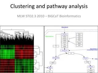
Clustering and Pathway Analysis. Lars Eijssen. Clustering and pathway analysis. Microarray analysis. Scanned microarrays. Image analysis. Raw intensities. QC, Normalization. Normalized intensities. Statistical analysis. Lists of regulated genes. Clustering. Pathway analysis.


Clustering and Pathway Analysis
E N D
Presentation Transcript
Clustering andPathway Analysis Lars Eijssen
Microarray analysis Scanned microarrays Image analysis Raw intensities QC, Normalization Normalized intensities Statistical analysis Lists of regulated genes Clustering Pathway analysis Pathway analysis Sets of co-regulated genes Sets of affected pathways Biological interpretation
Clustering and pathway analysis • Tools to help you interpret large datasets (e.g. microarray) • Clustering • Discover patterns in your data • Usually without prior knowledge (unsupervised) Find sets of genes that behave in a similar way • Pathway Analysis • Combine data with what we know about biology Find which and how biological processes are affected in your experiment
Contents • Background on Clustering Methods • Background on Pathway Analysis • Data Analysis with PathVisio • WikiPathways
Clustering • A cluster is a group that has homogeneity (internal cohesion) and separation (external isolation).
Clustering microarray data • High dimensional >10,000 measurements from relatively small number of samples • Use clustering to find groups of similar profiles • You can cluster on both samples and genes Image from J. Pennings, RIVM, NL
Quality control • As you have seen you can also use clustering for quality control Control group Hdh knockout group Zhang et al. BMC Neuroscience, 2008
How to compare data points? ? ? • Calculate a similarity measure • Commonly used similarity measures are • Pearson and Spearman correlation coefficients • Euclidean distance
Calculating Euclidean distance (I) • dpq is the distance between gene p and gene q • n is the number of samples • E.g. p1 is the measured expression of gene p, sample 1 a ya dab = ((xb – xa)2 + (yb – ya)2)1/2 yb b xa xb
Calculating Euclidean distance (II) • Watch out for measures on different scales • E.g.: weight in kg, length in cm, age in years • Important to standardize scales first: This can be done by: • subtracting the mean • dividing by the estimate of the standard deviation (s)
Pearson Distance • Based on Pearson correlation coefficient (1 - correlation) • Can capture inverse relations (for example, for genes that are inhibited)
Cluster algorithms • There are different cluster algorithms • Make use of similarity measure • Hierarchical • K-means • SOM • … and many more variations
Hierarchical clustering (I) • May be agglomerative … • building up the branches of a tree, beginning with the two most closely related objects • … or divisive • building the tree by finding the most dissimilar objects first • In each case, we end up with a clustering tree or dendrogramhaving branches and nodes.
a,b a,b,c,d,e c,d,e d,e Agglomerative 0 1 2 3 4 a b c d e Tree is constructed! Adapted from Kaufman and Rousseeuw (1990)
a a,b b c c,d,e d d,e e Divisive Tree is constructed! a,b,c,d,e 4 3 2 1 0 Adapted from Kaufman and Rousseeuw (1990)
1 12 Agglomerative and divisive clustering sometimes give conflicting results, as shown here 1 12
Hierarchical clustering (II) • How to compute the closest related items? • For step 1, simply the two items with the highest similarity (or smallest distance) are grouped first. • For the following steps we need to compute the (dis)similarity between groups of items • To compute this, several methods are available • In single-linkage clustering, the (dis)similarity between two groups of items is that of their most similar (less dissimilar) pair.
Hierarchical clustering methods (I) • There are many other criteria for defining clusters: • Single linkage • Complete linkage • Average linkage • Median linkage • Centroid linkage • Ward’s method • minimises variance single linkage complete linkage centroid linkage
Hierarchical clustering methods (II) • These do not always give equivalentclustering patterns • Average linkage and Ward’s methodseem most stable • Single-linkage clustering may besusceptible to ‘chaining’ of closelyrelated items, obscuring reasonablecluster structure chaining in single linkage
K-means clustering • Besides hierarchical methods many others are available • K-means clustering / Fuzzy K-means clustering • Choose number of clusters K • Take a random center for each cluster • Assign every item to the closest cluster • Recompute cluster centers (to be the average of all items it contains) • Re-assign items to the cluster of which the center is closest now • …and so on…until no change occurs any more • Advantage: easy method • Disadvantage: choice of K is arbitrarily – you still do not learn much about the relationships between the clusters (no dendrogram)
Kohonen Self Organising Maps (SOM) • Start with a ‘grid’ of MxN cluster centers • Train this grid to fit the data at hand • Clusters are linked to each other, if one cluster moves, it’s neigbhours also move a bit • Advantage: indicates relations between the clusters • Disadvantages: M and N arbitrarily – results not easy to interpret Image from J. Pennings, RIVM, NL
Clustering can supportBiological interpretation Two-way clustering of genes (y-axis) and cell lines (x-axis) (Alizadeh et al., 2000)
Free clustering software • TM4 MeVhttp://www.tm4.org/mev.html • Rhttp://www.r-project.org/ • Eisenhttp://rana.lbl.gov/EisenSoftware.htm • NCBI GEO also supports basic clustering:
Why Pathway Analysis? • Intuitive to biologists • Puts data in biological context • More intuitive way of looking at your data • More efficient than looking up gene-by-gene • Computational analysis • Overrepresentation analysis • Network analysis
Biological Context • Statistical results: • 1,300 genes are significantly regulated after treatment with X • Biological Meaning: • Is a certain biological pathway activated or deactivated? • Which genes in these pathway are significantly changed?
Pathway Collection • Where to get pathways? • Online pathway databases • WikiPathways www.wikipathways.org • Reactome www.reactome.org • Many more ... http://pathguide.org
Identifier Mapping Identifier Mapping Annotation: ENSG00000131828
Identifier Mapping • Microarrays typically use internal ids: • Affymetrix: 205749_at • Agilent: A_14_P106416 • Illumina: ILMN_4380 • Pathways typically use gene/protein ids • Entrez Gene: 1543 • Ensembl: ENSG00000140465 • UniProt: P04637
Identifier Mapping • 2 scenarios • Software will take care of it • e.g. PathVisio uses synonym databases • You will have to convert the ids yourself • DAVID: http://david.abcc.ncifcrf.gov • SOURCE: http://smd.stanford.edu/cgi-bin/source/sourceBatchSearch • BioMART: http://www.biomart.org • NetAffx: http://www.affymetrix.com
Pathway Analysis Tools • PathVisio • BioRAG • MetaCore (GeneGO) • Pathway-Express • GenMAPP / MAPPFinder
PathVisio www.pathvisio.org
Pathway Analysis Workflow Prepare your data Import your data in PathVisio Find „enriched“ pathways Visualize data on pathways Export pathway images
File Format • PathVisio accepts delimited text files • Prepare and export from Excel
File Format • Export from R write.table(myTable, file = txtFile, col.names = NA, sep = "\t", quote = FALSE, na = "NaN")
Identifier Systems PathVisio accepts many identifier systems: • Probes • Affymetrix, Illumina, Agilent,... • Genes and Proteins • Entrez Gene, Ensembl, UniProt, HUGO,... • Metabolites • ChEBI, HMDB, PubChem,...
Gene Database Your data A pathway Entrez Gene 5326 153 4357 65543 2094 90218 … 4357 ?? ENS0002114 P4235
Gene Database • Download from www.pathvisio.org/wiki/PathVisioDownload • 32 species supported
Exception File Exceptions file
Pgex File • Imported data is stored in a .pgex file • Load an existing dataset:
Statistics Unchanged gene Changed gene Question: • Does the small circle have a higher percentage of changed genes than the large circle? • Is this difference significant?
Calculate Z-scores • The Z-score can be used as a measure for how much a subset of genes is different from the rest • r = changed genes in Pathway • n = total genes in Pathway • R = changed genes • N = total genes Other enrichment calculation methods Ackermann M et al., A general modular framework for gene set enrichment analysis, BMC bioinformatics, 2009