Download
1 / 57
650 likes | 951 Vues
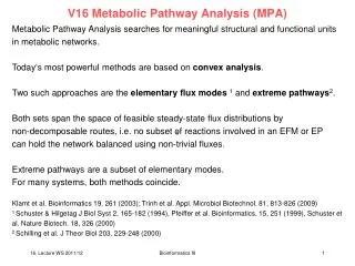
Metabolic Pathway Analysis. Fundamentals and Applications. Stefan Schuster Friedrich Schiller University Jena Dept. of Bioinformatics. Introduction. Analysis of metabolic systems requires theoretical methods due to high complexity

E N D
Metabolic Pathway Analysis. Fundamentals and Applications Stefan Schuster Friedrich Schiller University Jena Dept. of Bioinformatics
Introduction • Analysis of metabolic systems requires theoretical methods due to high complexity • Major challenge: clarify relationship between structure and function in complex intracellular networks • Study of robustness to enzyme deficiencies and knock-out mutations is of high medical and biotechnological relevance
Theoretical Methods • Dynamic Simulation • Stability and bifurcation analyses • Metabolic Control Analysis (MCA) • Metabolic Pathway Analysis • Metabolic Flux Analysis (MFA) • Optimization • and others
Theoretical Methods • Dynamic Simulation • Stability and bifurcation analyses • Metabolic Control Analysis (MCA) • Metabolic Pathway Analysis • Metabolic Flux Analysis (MFA) • Optimization • and others
Metabolic Pathway Analysis (or Metabolic Network Analysis) • Decomposition of the network into the smallest functional entities (metabolic pathways) • Does not require knowledge of kinetic parameters!! • Uses stoichiometric coefficients and reversibility/irreversibility of reactions
History of pathway analysis • „Direct mechanisms“ in chemistry (Milner 1964, Happel & Sellers 1982) • Clarke 1980 „extreme currents“ • Seressiotis & Bailey 1986 „biochemical pathways“ • Leiser & Blum 1987 „fundamental modes“ • Mavrovouniotis et al. 1990 „biochemical pathways“ • Fell (1990) „linearly independent basis vectors“ • Schuster & Hilgetag 1994 „elementary flux modes“ • Liao et al. 1996 „basic reaction modes“ • Schilling, Letscher and Palsson 2000 „extreme pathways“
Stoichiometry matrix Mathematical background • Example: 1 2 4 S S 1 2 3
Steady-state condition Balance equations for metabolites: dS/dt= NV(S) At any stationary state, this simplifies to: NV(S) = 0
Kernel of N Steady-state condition NV(S) = 0 If the kinetic parameters were known, this could be solved for S. If not, one can try to solve it for V. The equation system is linear in V. However, usually there is a manifold of solutions. Mathematically: kernel (null-space) of N. Spanned by basis vectors. These are not unique.
Use of null-space The basis vectors can be gathered in a matrix, K. They can be interpreted as biochemical routes across the system. If some row in K is a null row, the corresponding reaction is at thermodynamic equilibrium in any steady state of the system. Example: S 2 3 1 2 S P P 1 1 2
Use of null-space (2) It allows one to determine „enzyme subsets“ = sets of enzymes that always operate together at steady, in fixed flux proportions. The rows in K corresponding to the reactions of an enzyme subset are proportional to each other. Example: Enzyme subsets: {1,6}, {2,3}, {4,5} S 3 3 2 1 6 S S P P 4 1 1 2 5 4 S 2 Pfeiffer et al., Bioinformatics15 (1999) 251-257.
Drawbacks of null-space The basis vectors are not necessarily the simplest possible. They do not necessarily comply with the directionality of irreversible reactions. They do not always properly describe knock-outs. P 3 3 1 2 S P P 1 1 2
Drawbacks of null-space They do not always properly describe knock-outs. P 3 3 1 2 S P P 1 1 2 After knock-out of enzyme 1, the route {-2, 3} remains!
P S 4 3 non-elementary flux mode 1 1 P 1 3 S S 1 2 2 2 S 4 P P 1 2 P S 4 3 1 1 P 3 1 S S S S 1 2 1 2 1 1 1 1 S S 4 4 P P P P 1 2 1 2 elementary flux modes S. Schuster und C. Hilgetag: J. Biol. Syst. 2 (1994) 165-182
An elementary mode is a minimal set of enzymes that can operate at steady state with all irreversible reactions used in the appropriate direction The enzymes are weighted by the relative flux they carry. The elementary modes are unique up to scaling. All flux distributions in the living cell are non-negative linear combinations of elementary modes
Non-Decomposability property: For any elementary mode, there is no other flux vector that uses only a proper subset of the enzymesused by the elementary mode. For example, {HK, PGI, PFK, FBPase} is not elementary if {HK, PGI, PFK} is an admissible flux distribution.
Simple example: P 3 3 1 2 S P P 1 1 2 Elementary modes: They describe knock-outs properly.
Mathematical background (cont.) Steady-state condition NV = 0 Sign restriction for irreversible fluxes: Virr 0 This represents a linear equation/inequality system. Solution is a convex region. All edges correspond to elementary modes. In addition, there may be elementary modes in theinterior.
Geometrical interpretation Elementary modes correspond to generating vectors (edges) of a convex polyhedral cone (= pyramid) in flux space (if all modes are irreversible)
flux3 flux2 generating vectors flux1
If the system involves reversible reactions, there may be elementary modes in the interior of the cone. Example: P 3 3 1 2 S P P 1 1 2
Flux cone: There are elementary modes in the interior of the cone.
Pyr ATP X5P S7P E4P ADP Ru5P CO2 PEP NADPH GAP F6P R5P NADP 6PG 2PG 3PG GO6P ATP NADPH ADP NADP G6P F6P FP GAP 1.3BPG 2 NADH NAD DHAP ATP ADP Part of monosaccharide metabolism Red: external metabolites
Pyr ATP 2 ADP PEP 2 2PG 2 3PG ATP 2 ADP G6P F6P FP GAP 1.3BPG 2 2 NADH NAD DHAP ATP ADP 1st elementary mode: glycolysis
F6P FP 2 ATP ADP 2nd elementary mode: fructose-bisphosphate cycle
Pyr ATP X5P 2 S7P E4P 2 2 2 4 ADP Ru5P CO2 PEP NADPH GAP F6P 2 R5P 6 3 2 NADP 2 6PG 2PG 3 2 6 3PG GO6P ATP NADPH 2 6 3 ADP 5 NADP F6P FP GAP 1.3BPG G6P 2 2 2 NADH NAD DHAP ATP ADP 4 out of 7 elementary modes in glycolysis- pentose-phosphate system
Pyr X5P ATP 2 2 -4 4 1 S7P E4P 1 1 2 1 5 Ru5P 1 1 ADP 1 CO2 PEP -2 -2 1 NADPH 4 2 2 2 R5P GAP F6P 6 1 3 3 2 1 5 NADP 1 1 -2 2 6PG 6 1 2PG R5Pex 6 1 3 3 2 1 5 3PG GO6P ATP NADPH 2 1 5 6 1 3 3 -1 ADP 1 NADP 2 1 1 1 G6P F6P FP2 GAP 1.3BPG 1 1 2 2 1 -1 -2 1 5 5 DHAP NAD NADH -5 1 2 ATP 1 ADP 1 All 7 elementary modes in glycolysis- pentose-phosphate system S. Schuster, D.A. Fell, T. Dandekar: Nature Biotechnol. 18 (2000) 326-332
Optimization: Maximizing molar yields Pyr ATP X5P 2 S7P E4P 2 ADP Ru5P CO2 PEP NADPH GAP F6P R5P 3 2 NADP 6PG 2PG 3 2 3PG GO6P ATP NADPH 2 3 ADP NADP F6P FP GAP 1.3BPG G6P 2 2 2 NADH NAD DHAP ATP ADP ATP:G6P yield = 3ATP:G6P yield = 2
Synthesis of lysine in E. coli PG Pps Eno Pyk AceEF PEP Pyr AcCoA Ppc GltA AlaCon Cit Pck OAA Acn Ala Mdh Glu IlvE/AvtA AspC IsoCit Mal Gly Pyr Mas Icl Icd GluCon OG Fum Gdh Glu Succ AspCon AspA OG DapE Asp Fum Dia Sdh SucCD Sucdia ThrA Succ SucCoA SucAB DapF AspP CoA Glu YfdZ MDia Pyr DapA DapB Asd ASA Dpic Tpic Sucka LysA DapD LysCon Lysine(ext) Lysine
PG Elementary mode with the highest lysine : phosphoglycerate yield PEP Pyr (thick arrows: twofold value of flux) OAA Glu OG Glu Succ OG Asp Dia Sucdia Succ SucCoA AspP CoA MDia Pyr ASA Dpic Tpic Sucka Lysine(ext) Lysine
Maximization of tryptophan:glucose yield Model of 65 reactions in the central metabolism of E. coli. 26 elementary modes. 2 modes with highest tryptophan: glucose yield: 0.451. S. Schuster, T. Dandekar, D.A. Fell, Trends Biotechnol. 17 (1999) 53 Glc PEP 233 Pyr G6P Anthr 3PG PrpP GAP 105 Trp
Convex basis Minimal set of elementary modes sufficient to span the flux cone. Example: P 3 3 1 2 S P P 1 1 2
If the flux cone is pointed (all angles are less then 180o), then the convex basis is unique up to scaling. Otherwise, it is not. Example: Reactions 2 and 3 are reversible. P 3 S P P 1 1 2
For the latter example, the flux cone is a half-plane: The cone is not pointed. Again, there are elementary modes in the interior.
Related concept: Extreme pathways C.H. Schilling, D. Letscher and B.O. Palsson, J. theor. Biol. 203 (2000) 229 - distinction between internal and exchange reactions, all internal reversible reactions are split up into forward and reverse steps P S 4 3 P 3 S S 1 2 S 4 P P 1 2 Then, the convex basis is calculated. Spurious cyclic modes are discarded.
Advantages of extreme pathways: • Smaller number • Correspond to edges of flux cone • Drawbacks of extreme pathways: • Flux cone is higher-dimensional • Often not all relevant biochemical pathways represented • Knock-outs not properly described • Often route with maximal yield not covered • However, this depends on network configuration. • Originally, Schilling et al. (2000) proposed adding • exchange reaction for each external metabolite.
Network reconfiguration • Decomposition of internal reversible reactions into • forward and reverse steps • 2. Optionally: inclusion of (non-decomposed) • exchange reactions for each external metabolite. Now, there is a 1:1 correspondence between extreme pathways and elementary modes! P 3 S P P 1 1 2
Algorithm for computing elementary modes Related to Gauss-Jordan method Starts with tableau (NTI) Pairwise combination of rows so that one column of NT after the other becomes null vector
Example: S 2 3 4 1 2 S P P 1 1 2
These two rows should not be combined
Final tableau: S 2 3 4 1 2 S P P 1 1 2
Software for computing elementary modes EMPATH (in SmallTalk) - J. Woods METATOOL (in C) - Th. Pfeiffer, F. Moldenhauer, A. von Kamp, M. Pachkov Included in GEPASI - P. Mendes and JARNAC - H. Sauro part of METAFLUX (in MAPLE) -K. Mauch part of FluxAnalyzer (in MATLAB) -S. Klamt part of ScrumPy (in Python) - M. Poolman Alternative algorithm in MATLAB – C. Wagner (Bern) On-line computation: pHpMetatool - H. Höpfner, M. Lange http://pgrc-03.ipk-gatersleben.de/tools/phpMetatool/index.php
Combinatorial explosion of elementary modes A) S B) S 2*3 modes S external: 2+3 modes C) [S]
Proposed decomposition procedure • In addition to the pre-defined external metabolites, set all metabolites participating in more than 4 reactions to external status • Thus, the network disintegrates into subnetworks • Determine the elementary flux modes of the subnetworks separately
Mannitol Mycoplasma pneumoniae Subsystem 1 Sugar import Fructose Glucose Yellow boxes: additional external metabolites Subsystem 3 F6P R5P Nucleotide metab. Subsystem 2 PPP, glycolysis, dUMP dTMP fragm. lipid metab. Serine GA3P ATP Subsystem 5 C1 pool ADP Acetate Subsystem 4 Glycine Lower glycolysis Met f-Met CO2 Formate Subsystem 6 Ornithine NH3 Lactate Arginine Arginine degrad. Carbamate CO2
Robustness of metabolism • Number of elementary modes leading from a given substrate to a given product can be considered as a measure of redundancy • This is then also a rough estimate of robustness and of flexibility, because it characterizes the number of alternatives between which the network can switch if necessary
A) P 2 1 1 Q S 1 1 P 3 2 B) 2 1 S P 1 1 Q 1 S P 3 2 2 4 Number of elementary modes is not the best measure of robustness Knockout of enzyme 1 implies deletion of 2 elem. modes