Clustering Analysis
Clustering Analysis. CS 685: Special Topics in Data Mining Jinze Liu. Cluster Analysis. What is Cluster Analysis? Types of Data in Cluster Analysis A Categorization of Major Clustering Methods Partitioning Methods Hierarchical Methods Density-Based Methods Grid-Based Methods

Clustering Analysis
E N D
Presentation Transcript
Clustering Analysis CS 685: Special Topics in Data Mining Jinze Liu
Cluster Analysis • What is Cluster Analysis? • Types of Data in Cluster Analysis • A Categorization of Major Clustering Methods • Partitioning Methods • Hierarchical Methods • Density-Based Methods • Grid-Based Methods • Subspace Clustering/Bi-clustering • Model-Based Clustering
Inter-cluster distances are maximized Intra-cluster distances are minimized What is Cluster Analysis? • Finding groups of objects such that the objects in a group will be similar (or related) to one another and different from (or unrelated to) the objects in other groups
What is Cluster Analysis? • Cluster: a collection of data objects • Similar to one another within the same cluster • Dissimilar to the objects in other clusters • Cluster analysis • Grouping a set of data objects into clusters • Clustering is unsupervised classification: no predefined classes • Clustering is used: • As a stand-alone tool to get insight into data distribution • Visualization of clusters may unveil important information • As a preprocessing step for other algorithms • Efficient indexing or compression often relies on clustering
Some Applications of Clustering • Pattern Recognition • Image Processing • cluster images based on their visual content • Bio-informatics • WWW and IR • document classification • cluster Weblog data to discover groups of similar access patterns
What Is Good Clustering? • A good clustering method will produce high quality clusters with • high intra-class similarity • low inter-class similarity • The quality of a clustering result depends on both the similarity measure used by the method and its implementation. • The quality of a clustering method is also measured by its ability to discover some or all of the hidden patterns.
Requirements of Clustering in Data Mining • Scalability • Ability to deal with different types of attributes • Discovery of clusters with arbitrary shape • Minimal requirements for domain knowledge to determine input parameters • Able to deal with noise and outliers • Insensitive to order of input records • High dimensionality • Incorporation of user-specified constraints • Interpretability and usability
Outliers • Outliers are objects that do not belong to any cluster or form clusters of very small cardinality • In some applications we are interested in discovering outliers, not clusters (outlier analysis) cluster outliers
Data Structures attributes/dimensions • data matrix • (two modes) • dissimilarity or distance matrix • (one mode) tuples/objects the “classic” data input objects objects Assuming simmetric distance d(i,j) = d(j, i)
Measuring Similarity in Clustering • Dissimilarity/Similarity metric: • The dissimilarity d(i, j) between two objects i and j is expressed in terms of a distance function, which is typically a metric: • d(i, j)0 (non-negativity) • d(i, i)=0 (isolation) • d(i, j)= d(j, i) (symmetry) • d(i, j) ≤ d(i, h)+d(h, j) (triangular inequality) • The definitions of distance functions are usually different for interval-scaled, boolean, categorical, ordinal and ratio-scaled variables. • Weights may be associated with different variables based on applications and data semantics.
Type of data in cluster analysis • Interval-scaled variables • e.g., salary, height • Binary variables • e.g., gender (M/F), has_cancer(T/F) • Nominal (categorical) variables • e.g., religion (Christian, Muslim, Buddhist, Hindu, etc.) • Ordinal variables • e.g., military rank (soldier, sergeant, lutenant, captain, etc.) • Ratio-scaled variables • population growth (1,10,100,1000,...) • Variables of mixed types • multiple attributes with various types
Similarity and Dissimilarity Between Objects • Distance metrics are normally used to measure the similarity or dissimilarity between two data objects • The most popular conform to Minkowski distance: where i = (xi1, xi2, …, xin) and j = (xj1, xj2, …, xjn) are two n-dimensional data objects, and p is a positive integer • If p = 1, L1 is the Manhattan (or city block) distance:
Similarity and Dissimilarity Between Objects (Cont.) • If p = 2, L2is the Euclidean distance: • Properties • d(i,j) 0 • d(i,i)= 0 • d(i,j)= d(j,i) • d(i,j) d(i,k)+ d(k,j) • Also one can use weighted distance:
object j object i Binary Variables • A binary variable has two states: 0 absent, 1 present • A contingency table for binary data • Simple matching coefficient distance (invariant, if the binary variable is symmetric): • Jaccard coefficient distance (noninvariant if the binary variable is asymmetric): i= (0011101001) J=(1001100110)
Binary Variables • Another approach is to define the similarity of two objects and not their distance. • In that case we have the following: • Simple matching coefficient similarity: • Jaccard coefficient similarity: Note that: s(i,j) = 1 – d(i,j)
Dissimilarity between Binary Variables • Example (Jaccard coefficient) • all attributes are asymmetric binary • 1 denotes presence or positive test • 0 denotes absence or negative test
A simpler definition • Each variable is mapped to a bitmap (binary vector) • Jack: 101000 • Mary: 101010 • Jim: 110000 • Simple match distance: • Jaccard coefficient:
Variables of Mixed Types • A database may contain all the six types of variables • symmetric binary, asymmetric binary, nominal, ordinal, interval and ratio-scaled. • One may use a weighted formula to combine their effects.
Major Clustering Approaches • Partitioning algorithms: Construct random partitions and then iteratively refine them by some criterion • Hierarchical algorithms: Create a hierarchical decomposition of the set of data (or objects) using some criterion • Density-based: based on connectivity and density functions • Grid-based: based on a multiple-level granularity structure • Model-based: A model is hypothesized for each of the clusters and the idea is to find the best fit of that model to each other
Partitioning Algorithms: Basic Concept • Partitioning method: Construct a partition of a database D of n objects into a set of k clusters • k-means (MacQueen’67): Each cluster is represented by the center of the cluster • k-medoids or PAM (Partition around medoids) (Kaufman & Rousseeuw’87): Each cluster is represented by one of the objects in the cluster
K-means Clustering • Partitional clustering approach • Each cluster is associated with a centroid (center point) • Each point is assigned to the cluster with the closest centroid • Number of clusters, K, must be specified • The basic algorithm is very simple
K-means Clustering – Details • Initial centroids are often chosen randomly. • Clusters produced vary from one run to another. • The centroid is (typically) the mean of the points in the cluster. • ‘Closeness’ is measured by Euclidean distance, cosine similarity, correlation, etc. • Most of the convergence happens in the first few iterations. • Often the stopping condition is changed to ‘Until relatively few points change clusters’ • Complexity is O( n * K * I * d ) • n = number of points, K = number of clusters, I = number of iterations, d = number of attributes
Optimal Clustering Sub-optimal Clustering Two different K-means Clusterings Original Points
Evaluating K-means Clusters • For each point, the error is the distance to the nearest cluster • To get SSE, we square these errors and sum them. • x is a data point in cluster Ci and mi is the representative point for cluster Ci • can show that micorresponds to the center (mean) of the cluster • Given two clusters, we can choose the one with the smallest error
Solutions to Initial Centroids Problem • Multiple runs • Helps, but probability is not on your side • Sample and use hierarchical clustering to determine initial centroids • Select more than k initial centroids and then select among these initial centroids • Select most widely separated • Postprocessing • Bisecting K-means • Not as susceptible to initialization issues
Limitations of K-means • K-means has problems when clusters are of differing • Sizes • Densities • Non-spherical shapes • K-means has problems when the data contains outliers. Why?
The K-MedoidsClustering Method • Find representative objects, called medoids, in clusters • PAM (Partitioning Around Medoids, 1987) • starts from an initial set of medoids and iteratively replaces one of the medoids by one of the non-medoids if it improves the total distance of the resulting clustering • PAM works effectively for small data sets, but does not scale well for large data sets • CLARA (Kaufmann & Rousseeuw, 1990) • CLARANS (Ng & Han, 1994): Randomized sampling
PAM (Partitioning Around Medoids) (1987) • PAM (Kaufman and Rousseeuw, 1987), built in statistical package S+ • Use a real object to represent the a cluster • Select k representative objects arbitrarily • For each pair of a non-selected object h and a selected object i, calculate the total swapping cost TCih • For each pair of i and h, • If TCih < 0, i is replaced by h • Then assign each non-selected object to the most similar representative object • repeat steps 2-3 until there is no change
PAM Clustering: Total swapping cost TCih=jCjih • i is a current medoid, h is a non-selected object • Assume that i is replaced by h in the set of medoids • TCih = 0; • For each non-selected object j ≠ h: • TCih += d(j,new_medj)-d(j,prev_medj): • new_medj = the closest medoid to j after i is replaced by h • prev_medj = the closest medoid to j before i is replaced by h
j t t j h i h i h j i i h j t t PAM Clustering: Total swapping cost TCih=jCjih
CLARA (Clustering Large Applications) • CLARA (Kaufmann and Rousseeuw in 1990) • Built in statistical analysis packages, such as S+ • It draws multiple samples of the data set, applies PAM on each sample, and gives the best clustering as the output • Strength: deals with larger data sets than PAM • Weakness: • Efficiency depends on the sample size • A good clustering based on samples will not necessarily represent a good clustering of the whole data set if the sample is biased
CLARANS(“Randomized” CLARA) • CLARANS (A Clustering Algorithm based on Randomized Search) (Ng and Han’94) • CLARANS draws sample of neighbors dynamically • The clustering process can be presented as searching a graph where every node is a potential solution, that is, a set of k medoids • If the local optimum is found, CLARANS starts with new randomly selected node in search for a new local optimum • It is more efficient and scalable than both PAM and CLARA • Focusing techniques and spatial access structures may further improve its performance (Ester et al.’95)
Cluster Analysis • What is Cluster Analysis? • Types of Data in Cluster Analysis • A Categorization of Major Clustering Methods • Partitioning Methods • Hierarchical Methods • Density-Based Methods • Grid-Based Methods • Model-Based Clustering Methods • Outlier Analysis • Summary
Step 0 Step 1 Step 2 Step 3 Step 4 agglomerative (AGNES) a a b b a b c d e c c d e d d e e divisive (DIANA) Step 3 Step 2 Step 1 Step 0 Step 4 Hierarchical Clustering • Use distance matrix as clustering criteria. This method does not require the number of clusters k as an input, but needs a termination condition
AGNES (Agglomerative Nesting) • Implemented in statistical analysis packages, e.g., Splus • Use the Single-Link method and the dissimilarity matrix. • Merge objects that have the least dissimilarity • Go on in a non-descending fashion • Eventually all objects belong to the same cluster • Single-Link: each time merge the clusters (C1,C2) which are connected by the shortest single link of objects, i.e., minpC1,qC2dist(p,q)
A Dendrogram Shows How the Clusters are Merged Hierarchically Decompose data objects into a several levels of nested partitioning (tree of clusters), called a dendrogram. A clustering of the data objects is obtained by cutting the dendrogram at the desired level, then each connected component forms a cluster. E.g., level 1 gives 4 clusters: {a,b},{c},{d},{e}, level 2 gives 3 clusters: {a,b},{c},{d,e} level 3 gives 2 clusters: {a,b},{c,d,e}, etc. d e b a c level 4 level 3 level 2 level 1 a b c d e
DIANA (Divisive Analysis) • Implemented in statistical analysis packages, e.g., Splus • Inverse order of AGNES • Eventually each node forms a cluster on its own
More on Hierarchical Clustering Methods • Major weakness of agglomerative clustering methods • do not scale well: time complexity of at least O(n2), where n is the number of total objects • can never undo what was done previously • Integration of hierarchical with distance-based clustering • BIRCH (1996): uses CF-tree and incrementally adjusts the quality of sub-clusters • CURE (1998): selects well-scattered points from the cluster and then shrinks them towards the center of the cluster by a specified fraction • CHAMELEON (1999): hierarchical clustering using dynamic modeling
BIRCH (1996) • Birch: Balanced Iterative Reducing and Clustering using Hierarchies, by Zhang, Ramakrishnan, Livny (SIGMOD’96) • Incrementally construct a CF (Clustering Feature) tree, a hierarchical data structure for multiphase clustering • Phase 1: scan DB to build an initial in-memory CF tree (a multi-level compression of the data that tries to preserve the inherent clustering structure of the data) • Phase 2: use an arbitrary clustering algorithm to cluster the leaf nodes of the CF-tree • Scales linearly: finds a good clustering with a single scan and improves the quality with a few additional scans
Clustering Feature Vector Clustering Feature:CF = (N, LS, SS) N: Number of data points LS: Ni=1 Xi SS: Ni=1 (Xi )2 CF = (5, (16,30),244) (3,4) (2,6) (4,5) (4,7) (3,8)
Some Characteristics of CFVs • Two CFVs can be aggregated. • Given CF1=(N1, LS1, SS1), CF2 = (N2, LS2, SS2), • If combined into one cluster, CF=(N1+N2, LS1+LS2, SS1+SS2). • The centroid and radius can both be computed from CF. • centroid is the center of the cluster • radius is the average distance between an object and the centroid. Other statistical features as well...
CF-Tree in BIRCH • A CF tree is a height-balanced tree that stores the clustering features for a hierarchical clustering • A nonleaf node in a tree has (at most) B descendants or “children” • The nonleaf nodes store sums of the CFs of their children • A leaf node contains up to L CF entries • A CF tree has two parameters • Branching factor B: specify the maximum number of children. • threshold T: max radius of a sub-cluster stored in a leaf node
CF1 CF2 CF3 CF6 child1 child2 child3 child6 CF Tree (a multiway tree, like the B-tree) Root Non-leaf node CF1 CF2 CF3 CF5 child1 child2 child3 child5 Leaf node Leaf node prev CF1 CF2 CF6 next prev CF1 CF2 CF4 next
CF-Tree Construction • Scan through the database once. • For each object, insert into the CF-tree as follows: • At each level, choose the sub-tree whose centroid is closest. • In a leaf page, choose a cluster that can absort it (new radius < T). If no cluster can absorb it, create a new cluster. • Update upper levels.