Clustering Analysis
Clustering Analysis. Overview K-means Agglomerative Hierarchical Clustering DBSCAN Cluster Evaluation. Inter-cluster distances are maximized. Intra-cluster distances are minimized. What is Cluster Analysis?. [Chapter 8 . 1 . 1 , page 490].

Clustering Analysis
E N D
Presentation Transcript
Overview • K-means • Agglomerative Hierarchical Clustering • DBSCAN • Cluster Evaluation
Inter-cluster distances are maximized Intra-cluster distances are minimized What is Cluster Analysis? [Chapter 8 . 1 . 1 , page 490] • Finding groups of objects such that the objects in a group will be similar (or related) to one another and different from (or unrelated to) the objects in other groups • A good clustering method will produce high quality clusters with • high intra-cluster similarity • low inter-cluster similarity
Applications of Cluster Analysis [Chapter 8 . 1 . 1] • Understanding • Group related documents for browsing, group genes and proteins that have similar functionality, or group stocks with similar price fluctuations • Summarization • Reduce the size of large data sets Clustering precipitation in Australia
What is not Cluster Analysis? [Chapter 8 . 1 . 1 ] • Supervised classification • Have class label information • Simple segmentation • Dividing students into different registration groups alphabetically, by last name • Results of a query • Groupings are a result of an external specification • Graph partitioning • Some mutual relevance and synergy, but areas are not identical
How many clusters? Six Clusters Two Clusters Four Clusters Notion of a Cluster can be Ambiguous [Chapter 8 . 1 . 1]
Types of Clusterings [Chapter 8 . 1 . 2 , page 491] • A clustering is a set of clusters • Important distinction between hierarchical and partitionalsets of clusters • Partitional Clustering • A division data objects into non-overlapping subsets (clusters) such that each data object is in exactly one subset • Hierarchical clustering • A set of nested clusters organized as a hierarchical tree
A Partitional Clustering Partitional Clustering [Chapter 8 . 1 . 2 , page 491] Original Points
Hierarchical Clustering [Chapter 8 . 1 . 2 , page 492] Traditional Hierarchical Clustering Traditional Dendrogram Non-traditional Hierarchical Clustering Non-traditional Dendrogram
Other Distinctions Between Sets of Clusters [Chapter 8 . 1 . 2 , page 492] • Exclusive versus non-exclusive • In non-exclusive clusterings, points may belong to multiple clusters. • Can represent multiple classes or ‘border’ points • Fuzzy versus non-fuzzy • In fuzzy clustering, a point belongs to every cluster with some weight between 0 and 1 • Weights must sum to 1 • Probabilistic clustering has similar characteristics • Partial versus complete • In some cases, we only want to cluster some of the data • Heterogeneous versus homogeneous • Cluster of widely different sizes, shapes, and densities
Types of Clusters [Chapter 8 . 1 . 3 , page 493] • Well-separated clusters • Center-based clusters • Contiguous clusters • Density-based clusters • Property or Conceptual • Described by an Objective Function
Types of Clusters: Well-Separated [Chapter 8 . 1 . 3 , page 493] • Well-Separated Clusters: • A cluster is a set of points such that any point in a cluster is closer (or more similar) to every other point in the cluster than to any point not in the cluster. 3 well-separated clusters
Types of Clusters: Center-Based [Chapter 8 . 1 . 3 , page 494] • Center-based • A cluster is a set of objects such that an object in a cluster is closer (more similar) to the “center” of a cluster, than to the center of any other cluster • The center of a cluster is often a centroid, the average of all the points in the cluster, or a medoid, the most “representative” point of a cluster 4 center-based clusters
Types of Clusters: Contiguity-Based [Chapter 8 . 1 . 3 , page 494] • Contiguous Cluster (Nearest neighbor or Transitive) • A cluster is a set of points such that a point in a cluster is closer (or more similar) to one or more other points in the cluster than to any point not in the cluster. 8 contiguous clusters
Types of Clusters: Density-Based [Chapter 8 . 1 . 3 , page 494] • Density-based • A cluster is a dense region of points, which is separated by low-density regions, from other regions of high density. • Used when the clusters are irregular or intertwined, and when noise and outliers are present. 6 density-based clusters
Types of Clusters: Conceptual Clusters [Chapter 8 . 1 . 3 , page 495] • Shared Property or Conceptual Clusters • Finds clusters that share some common property or represent a particular concept. . 2 Overlapping Circles
Types of Clusters: Objective Function [optional] • Clusters Defined by an Objective Function • Finds clusters that minimize or maximize an objective function. • Enumerate all possible ways of dividing the points into clusters and evaluate the `goodness' of each potential set of clusters by using the given objective function. (NP Hard) • Can have global or local objectives. • Hierarchical clustering algorithms typically have local objectives • Partitional algorithms typically have global objectives • A variation of the global objective function approach is to fit the data to a parameterized model. • Parameters for the model are determined from the data. • Mixture models assume that the data is a ‘mixture' of a number of statistical distributions.
Types of Clusters: Objective Function … [optional] • Map the clustering problem to a different domain and solve a related problem in that domain • Proximity matrix defines a weighted graph, where the nodes are the points being clustered, and the weighted edges represent the proximities between points • Clustering is equivalent to breaking the graph into connected components, one for each cluster. • Want to minimize the edge weight between clusters and maximize the edge weight within clusters
Characteristics of the Input Data Are Important [optional] • Size • Scale • Normalization • Sparseness • Dictates type of similarity (proximity- type or density- type of measure) • Attribute type • Dictates type of similarity • Type of Data • Dictates type of similarity • Dimensionality • Noise and Outliers • Type of Distribution
Clustering Algorithms [Chapter 8 . 2 , page 496] • K-means and its variants • Hierarchical clustering • Density-based clustering
K-means Clustering [Chapter 8 . 2 . 1 , page 497] • Partitional clustering approach • Each cluster is associated with a centroid (center point) • Each point is assigned to the cluster with the closest centroid • Number of clusters, K, must be specified • The basic algorithm is very simple
K-means Clustering – Details [Chapter 8 . 2 . 1] • Initial centroids are often chosen randomly. • Clusters produced vary from one run to another. • The centroid is (typically) the mean of the points in the cluster. • ‘Closeness’ is measured by Euclidean distance, cosine similarity, correlation, etc. • K-means will converge for common similarity measures mentioned above. • Most of the convergence happens in the first few iterations. • Often the stopping condition is changed to ‘Until relatively few points change clusters’ • Complexity is O( n * K * I * d ) • n = number of points, K = number of clusters, I = number of iterations, d = number of attributes
Optimal Clustering Sub-optimal Clustering Two different K-means Clusterings [Chapter 8 . 2 . 1] Original Points
Importance of Choosing Initial Centroids [optional]
Importance of Choosing Initial Centroids [optional]
Squared Error 10 9 8 7 6 5 4 3 2 1 1 2 3 4 5 6 7 8 9 10 Objective Function Data mining and its applications
Evaluating K-means Clusters [Chapter 8 . 2 . 1 , page 499] • Most common measure is Sum of Squared Error (SSE) • For each point, the error is the distance to the nearest cluster • To get SSE, we square these errors and sum them. • x is a data point in cluster Ci and mi is the representative point for cluster Ci • can show that micorresponds to the center (mean) of the cluster • Given two clusterings, we can choose the one with the smallest error • One easy way to reduce SSE is to increase K, the number of clusters • A good clustering with smaller K can have a lower SSE than a poor clustering with higher K
Importance of Choosing Initial Centroids … [Chapter 8 . 2 . 1 , page 501]
Importance of Choosing Initial Centroids … [Chapter 8 . 2 . 1 , page 501]
K-Means Example Given: {2,4,10,12,3,20,30,11,25}, k=2 Data mining and its applications
Problems with Selecting Initial Points [Chapter 8 . 2 . 1 , page 503] • If there are K ‘real’ clusters then the chance of selecting one centroid from each cluster is small. • Chance is relatively small when K is large • If clusters are the same size, n, then • For example, if K = 10, then probability = 10!/1010 = 0.00036 • Sometimes the initial centroids will readjust themselves in ‘right’ way, and sometimes they don’t • Consider an example of five pairs of clusters
10 Clusters Example [optional] Starting with two initial centroids in one cluster of each pair of clusters
10 Clusters Example [Optional] Starting with two initial centroids in one cluster of each pair of clusters
10 Clusters Example [optional] Starting with some pairs of clusters having three initial centroids, while other have only one.
10 Clusters Example [optional] Starting with some pairs of clusters having three initial centroids, while other have only one.
Solutions to Initial Centroids Problem [Chapter 8 . 2 . 1 , page 504] • Multiple runs • Helps, but probability is not on your side • Sample and use hierarchical clustering to determine initial centroids • Select more than k initial centroids and then select among these initial centroids • Select most widely separated • Postprocessing • Bisecting K-means • Not as susceptible to initialization issues
Handling Empty Clusters [Chapter 8 . 2 . 2 , page 506] • Basic K-means algorithm can yield empty clusters • Several strategies • Choose the point that contributes most to SSE • Choose a point from the cluster with the highest SSE • If there are several empty clusters, the above can be repeated several times.
Updating Centers Incrementally [Chapter 8 . 2 . 2 , page 508] • In the basic K-means algorithm, centroids are updated after all points are assigned to a centroid • An alternative is to update the centroids after each assignment (incremental approach) • Never get an empty cluster • Can use “weights” to change the impact • Each assignment updates zero or two centroids • More expensive • Introduces an order dependency
Pre-processing and Post-processing [Chapter 8 . 2 . 2] • Pre-processing • Normalize the data • Eliminate outliers • Post-processing • To decrease the total SSE • Split ‘loose’ clusters, i.e., clusters with relatively high SSE • Introduce a ne cluster centroid • To decrease the number of clusters • Merge clusters that are ‘close’ or result in the smallest increase in total SSE • Eliminate small clusters that may represent outliers • Can use these steps during the clustering process
Bisecting K-means [Chapter 8 . 2 . 3, page 509] • Bisecting K-means algorithm • Variant of K-means that can produce a partitional or a hierarchical clustering
Bisecting K-means Example [Chapter 8 . 2 . 3]
Limitations of K-means [Chapter 8 . 2 . 4] • K-means has problems when clusters are of differing • Sizes • Densities • Non-globular shapes • K-means has problems when the data contains outliers.
Limitations of K-means: Differing Sizes [Chapter 8 . 2 . 4 , page 511] K-means (3 Clusters) Original Points
Limitations of K-means: Differing Density [Chapter 8 . 2 . 4 , page 511] K-means (3 Clusters) Original Points
Limitations of K-means: Non-globular Shapes [Chapter 8 . 2 . 4 , page 511] Original Points K-means (2 Clusters)
Overcoming K-means Limitations [Chapter 8 . 2 . 4_optional] Original Points K-means Clusters • One solution is to use many clusters. • Find parts of clusters, but need to put together.
Overcoming K-means Limitations [Chapter 8 . 2 . 4_optional] Original Points K-means Clusters
Overcoming K-means Limitations [Chapter 8 . 2 . 4_optional] Original Points K-means Clusters
Hierarchical Clustering [Chapter 8 . 3 , page 515-516] • Produces a set of nested clusters organized as a hierarchical tree • Can be visualized as a dendrogram • A tree like diagram that records the sequences of merges (or splits) dendrogram nested cluster diagram
Strengths of Hierarchical Clustering [chapter 8 . 3] • Do not have to assume any particular number of clusters • Any desired number of clusters can be obtained by ‘cutting’ the dendogram at the proper level • They may correspond to meaningful taxonomies • Example in biological sciences (e.g., animal kingdom, phylogeny reconstruction, …)