Power Linear Discriminant Analysis (PLDA)

1. Power Linear Discriminant Analysis (PLDA) M. Sakai, N. Kitaoka and S. Nakagawa, “Generalization of Linear Discriminant Analysis Used in Segmental Unit Input Hmm for Speech Recognition,” Proc. ICASSP, 2007 M. Sakai, N. Kitaoka and S. Nakagawa, “Selection of Optimal Dimensionality Reduction Method Using Chernoff Bound for Segmental Unit Input HMM,” Proc. INTERSPEECH, 2007 Reference: S. Nakagawa and K. Yamamoto, “Evaluation of Segmental Input Unit HMM,” Proc. ICASSP, 1996 K. Fukunaga, Introduction to Statistical Pattern Recognition, 2nd Ed. Presented by Winston Lee

2. M. Sakai, N. Kitaoka and S. Nakagawa, “Generalization of Linear Discriminant Analysis Used in Segmental Unit Input Hmm for Speech Recognition,” Proc. ICASSP, 2007

3. Abstract • To precisely model the time dependency of features is one of the important issues for speech recognition. Segmental unit input HMM with a dimensionality reduction method is widely used to address this issue. Linear discriminant analysis (LDA) and heteroscedastic discriminant analysis (HDA) are classical and popular approaches to reduce dimensionality. However, it is difficult to find one particular criterion suitable for any kind of data set in carrying out dimensionality reduction while preserving discriminative information. • In this paper, we propose a new framework which we call power linear discriminant analysis (PLDA). PLDA can describe various criteria including LDA and HDA with one parameter. Experimental results show that the PLDA is more effective than PCA, LDA, and HDA for various data sets.

4. Introduction • Hidden Markov Models (HMMs) have been widely used to model speech signals for speech recognition. However, HMMs cannot precisely model the time dependency of feature parameters. • Output-independent assumption of HMMs: All observations are dependent on the state that generated them, not on neighboring observations. • Segmental unit input HMM is widely (?) used to overcome this limitation. • In segmental unit input HMM, a feature vector is derived from several successive frames. The immediate use of several successive frames inevitably increases the dimensionality of parameters. • Therefore, a dimensionality reduction method is performed to spliced frames.

5. Segmental Unit Input HMM • The observation sequence The state sequence The expression of output probability computation of HMM is : Bayes’ Rule Bayes’ Rule Marginalizing

6. Segmental Unit Input HMM (cont.) conditional density HMM of 4-frame segments conditional density HMM of 2-frame segments segmental unit input HMM of 2-frame segments the standard HMM

7. Segmental Unit Input HMM (cont.) • The segmental unit input HMM in (Nakagawa, 1996) is approximation of • Using segmental unit input HMM wherein several successive frames are inputted as one vector, since the dimensions of vector increases, it results in a lesser precision in the estimation of the covariance matrix. • In (Nakagawa, 1996), Karhunen-Loeve (K-L) expansion and Modified Quadratic Discriminant Function (MQDF) are used to deal with the above problem. segmental unit input HMM of 4-frame segments

8. K-L Expansion • Estimation of covariance matrix from samples • Computation of eigenvalues and eigenvectors • Sort of eigenvalues and eigenvectors corresponding to them: • Computation of parameters having compressed dimension, by usingwhere the transformation matrix is as follows

9. K-L Expansion (cont.) • In the statistical literature, K-L expansion is generally called principal components analysis (PCA). • Some criteria of K-L expansion: • minimum mean-square error (MMSE) • maximum scatter measure • minimum entropy • Remarks: • Why orthonormal linear transformations?Ans: To maintain the structure of the distribution.

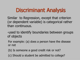
10. Review on LDA • Given n-dimensional features e.g., let us find a transformation matrix that maps these features to p-dimensional features where and N denotes the number of features. • Within-class covariance matrices: • Between-class covariance matrices:

11. Review on LDA (cont.) • In LDA, the objective function is defined as follows: • LDA finds a transformation matrix B that maximizes the above function. • The eigenvectors corresponding to the largest eigenvalues of are the solution.

12. Review on HDA • LDA is not the optimal transform when the class distributions are heteroscedastic. • HLDA: Kumar incorporated the maximum likelihood estimation of parameters for differently distributed Gaussians. • HDA: Saon proposed another objective function similar to Kumar’s and showed its relationship with a constrained maximum likelihood estimation. • Saon’s HDA objective function:

13. Dependency on Data Set • Figure 1(a) shows that HDA has higher separability than LDA for the data set. • Figure 1(b) shows that LDA has higher separability than HDA for another data set. • Figure 1(c) shows the case with another data set where both LDA and HDA have low separabilities. • All results show that the separabilities of LDA and HDA depend significantly on data sets.

14. Dependency on Data Set (cont.)

15. Relationship between LDA and HDA • The denominator in Eq. (1) can be viewed as a determinant of the weighted arithmetic mean of the class covariance matrices. • The denominator in Eq. (2) can be viewed as a determinant of the weighted geometric mean of the class covariance matrices.

16. PLDA • The difference between LDA and HDA is the definitions of the mean of the class covariance matrices. • As extension of this interpretation, their denominators can be replaced by a determinant of the weighted harmonic mean, or a determinant of the root mean square, etc. • In this paper, a more general definition of a mean is often used, called the weighted mean of order m, or the weighted power mean. • The new approach using the weighted power mean as the denominator of the objective function is called Power Linear Discriminant Analysis (PLDA).

17. PLDA (cont.) • The new objective function is as follows: • It can be seen that both of LDA and HDA are the subsets of PLDA. • m=1 (arithmetic mean) • m=0 (geometric mean)

18. Appendix A • weighted power mean: • If are positive real numbers such that we define the r-th weighted power mean of the as:

19. Appendix B • Let we want to find • First we take logarithm of : • Then • So l’Hôpital’s rule

20. PLDA (cont.) • Assuming that a control parameter m is constrained to be an integer, the derivatives of the PLDA objective function are formulated as follows:

21. Appendix C • m > 0

22. Appendix C (cont.) • m = 0 (too trivial!) • m < 0

23. The Diagonal Case • Because of computational simplicity, the covariance matrix in the class k is often assumed to be diagonal. • Since a diagonal matrix multiplication is commutative, the derivatives of the PLDA objective function are simplified as follows:

24. Experiments • Corpus: CENSREC-3 • The CENSREC-3 is designed as an evaluation framework of Japanese isolated word recognition in real driving car environments. • Speech data was collected using 2 microphones, a close-talking (CT) microphone and a hands-free (HF) microphone. • For training, a total of 14,050 utterances spoken by 293 drivers (202 males and 91 females) were recorded with both microphones. • For evaluation, a total of 2,646 utterances spoken by 18 speakers (8 males and 10 females) were evaluated for each microphone.

25. Experiments (cont.)

26. P.S. • Apparently, the deviation of PLDA is merely an induction from LDA and HDA. • The authors doesn’t seem to give any expressive statistical or physical meaning about PLDA. • The experimental results shows PLDA (with some parameter m) overperforms the other two approaches, but it does not explained why in this paper. • The revised version of Fisher’s criterion!!!!! • The concepts of MEAN!!!!!

27. M. Sakai, N. Kitaoka and S. Nakagawa, “Selection of Optimal Dimensionality Reduction Method Using Chernoff Bound for Segmental Unit Input HMM,” Proc. INTERSPEECH, 2007

28. Abstract • To precisely model the time dependency of features, segmental unit input HMM with a dimensionality reduction method has been widely used for speech recognition. Linear discriminant analysis (LDA) and heteroscedastic discriminant analysis (HDA) are popular approaches to reduce the dimensionality. We have proposed another dimensionality reduction method called power linear discriminant analysis (PLDA) to select the best dimensionality reduction method that yields the highest recognition performance. This selection process on the basis of trial and error requires much time to train HMMs and to test the recognition performance for each dimensionality reduction method. • In this paper we propose a performance comparison method without training or testing. We show that the proposed method using the Chernoff bound can rapidly and accurately evaluate the relative recognition performance.

29. Performance Comparison Method • Instead of using a recognition error, The class separability error of the features in the projected space is used as a criterion to estimate the parameter m of PLDA.

30. Performance Comparison Method (cont.) • Two-class problem: • Bayes error of the projected features on an evaluation data: • The Bayes error ε can represent a classification error, assuming that the training data and the evaluation data come from the same distributions. • But, it’s hard to measure the Bayes error.

31. Performance Comparison Method (cont.) • Two-class problem (cont.): • Instead, we use the Chernoff bound between class 1 and class 2 as a class separability error • We can rewrite the above equation aswhere s = 0.5: Bhattacharyya bound Covariance matrices are treated as diagonal ones here

32. Performance Comparison Method (cont.)

33. Performance Comparison Method (cont.) • Multi-class problem: • it is possible to define several error functions for multi-class data. • Sum of pairwise approximated errors: • Maximum pairwise approximated error

34. Performance Comparison Method (cont.) • Multi-class problem (cont.): • Sum of maximum approximated errors in each class

35. Experimental Results

36. Experimental Results (cont.)

37. Experimental Results (cont.) • No comparison method could predict the best dimensionality reduction methods simultaneously for both of the two evaluation sets. • It is supposed that this results from neglecting time information of speech feature sequences to measure a class separability error and modeling a class distribution as a unimodal normal distribution. • Computational costs

38. P.S. • The experimental results didn’t explicitly explain the relationship between WER and class separatability error for a given m. That is, better class separatability error cannot explicitly guarantee better WER. (The authors said, they “agree well”.) • In the experiment, the authors didn’t explain the differences among the three criteria when calculating approximated errors. • But this is a good try to take something out from the black boxes (WERs).