Discriminant Function Analysis
Discriminant Function Analysis. Mechanics. Equations. To get our results we’ll have to use those same SSCP matrices as we did with Manova. Equations.

Discriminant Function Analysis
E N D
Presentation Transcript
Discriminant Function Analysis Mechanics
Equations • To get our results we’ll have to use those same SSCP matrices as we did with Manova
Equations • The diagonals for the matrices are the sums of squared deviations about means for that variable, while the offdiagonals contain the cross-products of those deviations for the variables involved
The eigenvalues and eigenvectors will again be found for the BW-1 matrix as in Manova • We will use the eigenvectors (vi) to come to our eventual coefficients used in the linear combination of DVs • The discriminant score for a given case represents the position of that case along the continuum (axis) defined by that function • In the original our new axes (dimensions, functions) could be anywhere, but now will have an origin coinciding with the grand centroid (where all the means of the DVs meet)
Equations • Our original equation here in standardized form • a standardized discriminant function score ( ) equals the standardized scores times its standardized discriminant function coefficient ( )
Note that we can label our coefficients in the following fashion • Raw – vi • From eigenvectors • Not really interpretable as coefficients and have no intrinsic meaning as far as the scale is concerned • Unstandardized - ui • Actually are in a standard score form (mean = 0, within groups variance = 1) • Discriminant scores represent distance in standard deviation units, from the grand centroid • Standardized – di • uis for standardized data • Allow for a determination of relative importance
Classification • Classification score for group j is found by multiplying the raw score on each predictor (x) by its associated classification function coefficient (cj), summing over all predictors and adding a constant, cj0
Equations • The coefficients are found by taking the inverse of the within subjects variance-covariance matrix W (just our usual SSCP matrix values divided by within groups df [N-k]) and multiplying it by the column vector of predictor means: • and the intercept is found by: Where Cj is the row vector of coefficients. A 1 x m vector times a q x 1 vector results in a scalar (single value)
Prior probability • The adjustment is made to the classification function by adding the natural logarithm of the prior probability for that group to the constant term • or subtracting 2 X this value from the Mahalanobis’ distance • Doing so will make little difference with very distinct groups, but can in situations where there is more overlap • Note that this should only be done for theoretical reasons • If a strong one cannot be found, one is better of not messing with it