Logistic Regression and Discriminant Function Analysis

1. Logistic Regression and Discriminant Function Analysis

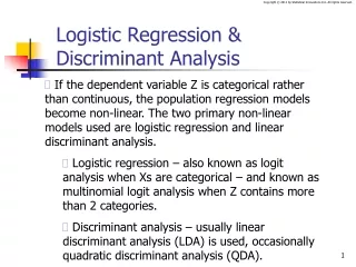
2. Logistic Regression vs. Discriminant Function Analysis • Similarities • Both predict group membership for each observation (classification) • Dichotomous DV • Requires an estimation and validation sample to assess predictive accuracy • If the split between groups is not more extreme than 80/20, yield similar results in practice

3. Logistic Reg vs. Discrim: Differences • Discriminant Analysis • Assumes MV normality • Assumes equality of VCV matrices • Large number of predictors violates MV normality can’t be accommodated • Predictors must be continuous, interval level • More powerful when assumptions are met • Many assumptions, rarely met in practice • Categorical IVs create problems • Logistic Regression • No assumption of MV normality • No assumption of equality of VCV matrices • Can accommodate large numbers of predictors more easily • Categorical predictors OK (e.g., dummy codes) • Less powerful when assumptions are met • Few assumptions, typically met in practice • Categorical IVs can be dummy coded

4. Logistic Regression • Outline: • Categorical Outcomes: Why not OLS Regression? • General Logistic Regression Model • Maximum Likelihood Estimation • Model Fit • Simple Logistic Regression

5. Categorical Outcomes: Why not OLS Regression? • Dichotomous outcomes: • Passed / Failed • CHD / No CHD • Selected / Not Selected • Quit/ Did Not Quit • Graduated / Did Not Graduate

6. Categorical Outcomes: Why not OLS Regression? • Example: Relationship b/w performance and turnover • Line of best fit?! • Errors (Y-Y’) across • values of performance (X)?

7. Problems with Dichotomous Outcomes/DVs • The regression surface is intrinsically non-linear • Errors assume one of two possible values, violate assumption of normally distributed errors • Violates assumption of homoscedasticity • Predicted values of Y greater than 1 and smaller than 0 can be obtained • The true magnitude of the effects of IVs may be greatly underestimated • Solution: Model data using Logistic Regression, NOT OLS Regression

8. Logistic Regression vs. Regression • Logistic regression predicts a probability that an event will occur • Range of possible responses between 0 and 1 • Must use an s-shaped curve to fit data • Regression assumes linear relationships, can’t fit an s-shaped curve • Violates normal distribution • Creates heteroscedascity

9. Example: Relationship b/w Age and CHD (1 = Has CHD)

10. General Logistic Regression Model • Y’ (outcome variable) is the probability that having one outcome or another based on a nonlinear function of the best linear combination of predictors Where: • Y’ = probability of an event • Linear portion of equation (a + b1x1) used to predict probability of event (0,1), not an end in itself

11. The logistic (logit) transformation • DV is dichotomous purpose is to estimate probability of occurrences (0, 1) • Thus, DV is transformed into a likelihood • Logit/logistic transformation accomplishes (linear regression eq. takes log of odds)

12. Probability Calculation Where: The relation b/w logit (P) and X is intrinsically linear b = expected change of logit(P) given one unit change in X a = intercept e = Exponential

13. Ordinary Least Squares (OLS) Estimation • Purpose is obtain the estimates that would best minimize the sum of squared errors, sum(y-y’)2 • The estimates chosen best describe the relationships among the observed variables (IVs and DV) • Estimates chosen maximize the probability of obtaining the observed data (i.e., these are the population values most likely to produce the data at hand)

14. Maximum Likelihood (ML) estimation • OLS can’t be used in logistic regression because of non-linear nature of relationships • In ML, the purpose is to obtain the parameter estimates most likely to produce the data • ML estimators are those with the greatest joint likelihood of reproducing the data • In logistic regression, each model yields a ML joint probability (likelihood) value • Because this value tends to be very small (e.g., .00000015), it is multiplied by -2log • The -2log transformation also yields a statistic with a known distribution (chi-square distribution)

15. Model Fit • In Logistic Regression, R & R2 don’t make sense • Evaluate model fit using the -2log likelihood (-2LL) value obtained for each model (through ML estimation) • The -2LL value reflects fit of model; used to compare fit of nested models • The -2LL measures lack of fit – extent to which model fits data poorly • When the model fits the data perfectly, -2LL = 0 • Ideally, the -2LL value for the null model (i.e., model with no predictors, or “intercept-only” model) would be larger than then the model with predictors

16. Comparing Model Fit • The fit of the null model can be tested against the fit of the model with predictors using chi-square test: Where: • 2 = chi-square for improvement in model fit (where df = kNull – kModel) • -2LLMO = -2 Log likelihood value for null model (intercept-only model) • -2LLM1 = -2 Log likelihood value for hypothesized model • Same test can be used to compare nested model with k predictor(s) to model with k+1 predictors, etc. • Same logic as OLS regression, but the models are compared using a different fit index (-2LL)

17. Pseudo R2 • Assessment of overall model fit • Calculation • Two primary Pseudo R2 stats: • Nagelkerke less conservative • preferred by some because max = 1 • Cox & Snell more conservative • Interpret like R2 in OLS regression

18. Unique Prediction • In OLS regression, the significance tests for the beta weights indicate if the IV is a unique predictors • In Logistic regression, the Wald test is used for the same purpose

19. Similarities to Regression • You can use all of the following procedures you learned about OLS regression in logistic regression • Dummy coding for categorical IVs • Hierarchical entry of variables (compare changes in % classification; significance of Wald test) • Stepwise (but don’t use, its atheoretical) • Moderation tests

20. Simple Logistic Regression Example • Data collected from 50 employees • Y = success in training program (1 = pass; 0 = fail) • X1 = Job aptitude score (5 = very high; 1= very low) • X2 = Work-related experience (months)

21. Syntax in SPSS DV LOGISTIC REGRESSION PASS /METHOD = ENTER APT EXPER /SAVE = PRED PGROUP /CLASSPLOT /PRINT = GOODFIT /CRITERIA = PIN(.05) POUT(.10) ITERATE(20) CUT(.5) . IVs

22. Results • Block O: The Null Model results • Can’t do any worse than this • Block 1: Method = Enter • Tests of the model of interest • Interpret data from here Tests if model is significantly better than the null model. Significant chi-square means yes! Step, Block & Model yield same results because all IVs entered in same block

23. Results Continued -2 Log Likelihood an index of fit - smaller number means better fit (Perfect fit = 0) Pseudo R2 – Interpret like R2 in regression Nagelkerke preferred by some because max = 1, Cox & Snell more conservative estimate uniformly

24. Classification: Null Model vs. Model Tested Null Model 52% correct classification Model Tested 72% correct classification

25. Variables in Equation B  effect of one unit change in IV on the log odds (hard to interpret) *Odds Ratio (OR)  Exp(B) in SPSS = more interpretable; one unit change in aptitude increases the probability of passing by 1.7x Wald  Like t test, uses chi-square distribution Significance  to determine if wald test is significant

26. Histogram of Predicted Probabilities

27. To Flag Misclassified Cases SPSS syntax COMPUTE PRED_ERR=0. IF LOW NE PGR_1 PRED_ERR=1. You can use this for additional analyses to explore causes of misclassification

28. Results Continued An index of model fit. Chi-square compares the fit of the data (the observed events) with the model (the predicted events). The n.s. results means that the observed and expected values are similar  this is good!

29. Hierarchical Logistic Regression • Question: Which of the following variables predict whether a woman is hired to be a Hooters girl? • Age • IQ • Weight

30. Simultaneous v. Hierarchical Block 1. IQ Block 1. IQ, Age, Weight Cox & Snell .002; Nagelkerke .003 Block 2. Age Cox & Snell .264; Nagelkerke .353 Block 3. Weight Cox & Snell .296; Nagelkerke .395

31. Simultaneous v. Hierarchical Block 1. IQ Block 1. IQ, Age, Weight Block 2. Age Block 3. Weight

32. Simultaneousv. Hierarchical Block 1. IQ Block 1. IQ, Age, Weight Block 2. Age Block 3. Weight

33. Multinomial Logistic Regression • A form of logistic regression that allows prediction of probability into more than 2 groups • Based on a multinomial distribution • Sometimes called polytomous logistic regression • Conducts an omnibus test first for each predictor across 3+ groups (like ANOVA) • Then conduct pairwise comparisons (like post hoc tests in ANOVA)

34. Objectives of Discriminant Analysis • Determining whether significant differences exist between average scores on a set of variables for 2+ a priori defined groups • Determining which IVs account for most of the differences in average score profiles for 2+ groups • Establishing procedures for classifying objects into groups based on scores on a set of IVs • Establishing the number and composition of the dimensions of discrimination between groups formed from the set of IVs

35. Discriminant Analysis • Discriminant analysis develops a linear combination that can best separate groups. • Opposite of MANOVA • In MANOVA, groups are usually constructed by researcher and have clear structure (e.g., a 2 x 2 factorial design). Groups = IVs • In discriminant analysis, the groups usually have no particular structure and their formation is not under experimental control. Groups = DVs

36. How Discrim Works • Linear combinations (discriminant functions) are formed that maximize the ratio of between-groups variance to within-groups variance for a linear combination of predictors. • Total # discriminant functions = # groups – 1 OR # of predictors (whichever is smaller) • If more than one discriminant function is formed, subsequent discriminant functions are independent of prior combinations and account for as much remaining group variation as possible.

37. Assumptions in Discrim • Multivariate normality of IVs • Violation more problematic if overlap between groups • Homogeneity of VCV matrices • Linear relationships • IVs continuous (interval scale) • Can accommodate nominal but violates MV normality • Single categorical DV Results influenced by: • Outliers (classification may be wrong) • Multicollinearity (interpretation of coefficients difficult)

38. Sample Size Considerations • Observations: # Predictors • Suggested 20 observations per predictor • Minimum required 5 observations per predictor • Observations: Groups (in DV) • Minimum: smallest group size exceeds # of IVs • Practical Guide: Each group should have 20+ observations • Wide variation in group size impacts results (i.e., classification is incorrect)

39. Example In this hypothetical example, data from 500 graduate students seeking jobs were examined. Available for each student were three predictors: GRE(V+Q), Years to Finish the Degree, and Number of Publications. The outcome measure was categorical: “Got a job” versus “Did not get a job.” Half of the sample was used to determine the best linear combination for discriminating the job categories. The second half of the sample was used for cross-validation.

40. DISCRIMINANT /GROUPS=job(1 2) /VARIABLES=gre pubs years /SELECT=sample(1) /ANALYSIS ALL /SAVE=CLASS SCORES PROBS /PRIORS SIZE /STATISTICS=MEAN STDDEV UNIVF BOXM COEFF RAW CORR COV GCOV TCOV TABLE CROSSVALID /PLOT=COMBINED SEPARATE MAP /PLOT=CASES /CLASSIFY=NONMISSING POOLED .

47. Interpreting Output • Box’s M • Eigenvalues • Wilks Lambda • Discriminant Weights • Discriminant Loadings

49. Violates Assumption of Homogeneity of VCV matrices. But this test is sensitive in general and sensitive to violations of multivariate normality too. Tests of significance in discriminant analysis are robust to moderate violations of the homogeneity assumption.