Multiple Discriminant Analysis and Logistic Regression
260 likes | 473 Vues
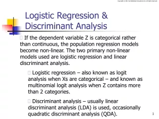
Multiple Discriminant Analysis and Logistic Regression. Multiple Discriminant Analysis. Appropriate when dep. var. is categorical and indep. var. are metric MDA derives variate that best distinguishes between a priori groups

Multiple Discriminant Analysis and Logistic Regression
E N D
Presentation Transcript
Multiple Discriminant Analysis • Appropriate when dep. var. is categorical and indep. var. are metric • MDA derives variate that best distinguishes between a priori groups • MDA sets variate’s weights to maximize between-group variance relative to within-group variance
MDA • For each observation we can obtain a Discriminant Z-score • Average Z score for a group gives Centroid • Classification done using Cutting Scores which are derived from group centroids • Statistical significance of Discriminant Function done using distance bet. group centroids • LR similar to 2-group discriminant analysis
The MDA Model • Six-stage model building for MDA • Stage 1: Research problem/Objectives a. Evaluate differences bet. avg. scores for a priori groups on a set of variables b. Determine which indep. variables account for most of the differences bet. groups c. Classify observations into groups
The MDA Model • Stage 2: Research design a. Selection of dep. and indep. variables b. Sample size considerations c. Division of sample into analysis and holdout sample
The MDA Model • Stage 3: Assumptions of MDA a. Multivariate normality of indep. var. b. Equal Covariance matrices of groups c. Indep. vars. should not be highly correlated. d. Linearity of discriminant function • Stage 4: Estimation of MDA and assessing fit a. Estimation can be i. Simultaneous ii. Stepwise
The MDA Model • Step 4: Estimation and assessing fit (contd) b. Statistical significance of discrim function i. Wilk’s lambda, Hotelling’s trace, Pillai’s criterion, Roy’s greatest root ii. For stepwise method, Mahalanobis D2 , iii. Test stat sig. of overall discrimination between groups and of each discriminant function
MDA and LR (contd) • Step 4: Estimation and assessing fit (contd) c. Assessing overall fit i. Calculate discrim. Z-score for each obs. ii. Evaluate group differences on Z scores iii. Assess group membership prediction accuracy. To do this we need to address following - rationale for classification matrices
The MDA Model • Step 4: Estimation and assessing fit (contd) c. Assessing overall fit(contd.) iii. Address the following (contd.) - cutting score determination - consider costs of misclassification - constructing classification matrices - assess classification accuracy - casewise diagnostics
The MDA Model • Stage 5: Interpretation of results a. Methods for single discrim. function i. Discriminant weights ii. Discriminant loadings iii. Partial F-values b. Additional methods for more than 2 functions i. Rotation of discrim. functions ii. Potency index iii. Stretched attribute vectors
The MDA Model • Stage 6: Validation of results
Logistic Regression • For 2 groups LR is preferred to MDA because 1. More robust to failure of MDA assumptions 2. Similar to regression, so intuitively appealing 3. Has straightforward statistical tests 4. Can accommodate non-linearity easily 5. Can accommodate non-metric indep var. through dummy variable coding
The LR Model • Six stage model building for LR • Stage 1: Research prob./objectives (same as MDA) • Stage 2: Research design (same as MDA) • Stage 3: Assumptions of LR (same as MDA) • Stage 4: Estimating LR and assessing fit a. Estimation uses likelihood of an event’s occurrence
The LR Model • Stage 4: Estimating LR and assessing fit (contd) b. Assessing fit i. Overall measure of fit is -2LL ii.Calculation of R2 for Logit iv. Assess predictive accuracy
The LR Model • Step 5: Interpretation of results a. Many MDS methods can be used b. Test significance of coefficients • Step 6: Validation of results
Example: Discriminant Analysis • HATCO is a large industrial supplier • A marketing research firm surveyed 100 HATCO customers • There were two different types of customers: Those using Specification Buying and those using Total Value Analysis • HATCO mgmt believes that the two different types of customers evaluate their suppliers differently
Example: Discriminant Analysis • In a B2B situation, HATCO wanted to know the perceptions that its customers had about it • The mktg res firm gathered data on 7 variables 1. Delivery speed 2. Price level 3. Price flexibility 4. Manufacturer’s image 5. Overall service 6. Salesforce image 7. Product quality • Each var was measured on a 10 cm graphic rating scale Poor Excellent
Example: Discriminant Analysis • Stage 1: Objectives of Discriminant Analysis Which perceptions of HATCO best distinguish firms using each buying approach? • Stage 2: Research design a. Dep var is the buying approach of customers. It is categorical. Indep var are X1 to X7 as mentioned above b. Overall sample size is 100. Each group exceeded the minimum of 20 per group c. Analysis sample size was 60 and holdout sample size was 40
Example: Discriminant Analysis • Stage 3: Assumptions of MDA All the assumptions were met • Stage 4: Estimation of MDA and assessing fit Before estimation, we first examine group means for X1 to X7 and the significances of difference in means a. Estimation is done using the Stepwise procedure. - The indep var which has the largest Mahalanobis D2 distance is selected first and so on, till none of the remaining var are significant - The discriminant function is obtained from the unstandardized coefficients
Example: Discriminant Analysis • Stage 4: Estimation of MDA and assessing fit (cont) b. Univariate and multivariate aspects show significance c. Discrim Z-score for each observation and group centriods were calculated - The cutting score was calculated nA=Number in Group A (Total Value Analysis) nB=Number in Group B (Specification Buying) zA=Centroid of Group A zB=Centroid of Group B Cutting Score, zC= (nAzB+nBzA)/(nA+nB)
Example: Discriminant Analysis • Stage 4: - The cutting score was calculated as -0.773 - Classification matrix was calculated by classifying an observation as Specification buying/Total value analysis if it’s Z-score was less/greater than –0.773 - Classification accuracy was obtained and assessed using certain benchmarks
Example: Discriminant Analysis • Step 5: Interpretation -Since we have a single discriminant function, we will look at the discriminant weights, loadings and partial F values - Discriminant loadings are more valid for interpretation. We see that X7 discriminates the most followed by X1 and then X3 - Going back to table of group means, we see that firms employing Specification Buying focus on ‘Product quality’, whereas firms using Total Value Analysis focus on ‘Delivery speed’ and ‘Price flexibility’ in that order
Example: Logistic Regression • A cataloger wants to predict response to mailing • Draws sample of 20 customers • Uses three variables - RESPONSE (0=no/1=yes) the dep var - AGE (in years) an indep var - GENDER (0=male/1=female) an indep var • Use Dummy variables for categorical variables
Example: Logistic Regression • Running the logistic regression program gives G = -10.83 + .28 AGE +2.30 GENDER • Here G is the Logit of a yes response to mailing • Consider a male of age 40. His G or logit score is G(0, 40) = -10.83 + .28*40 + 2.30*0 = .37 logit • A female customer of same age would have G(1, 40) = -10.83 + .28*40 + 2.30*1 = 2.67 logits • Logits can be converted to Odds which can be converted to probabilities • For the 40 year old male/female prob is p = .59/.93