Multiple Regression Analysis
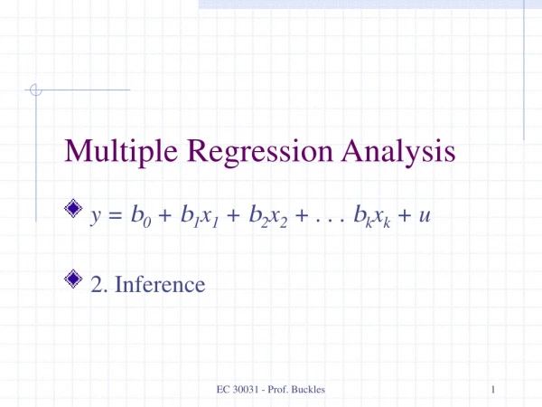
Multiple Regression Analysis. y = b 0 + b 1 x 1 + b 2 x 2 + . . . b k x k + u 3. Asymptotic Properties. Consistency. Under the Gauss-Markov assumptions OLS is BLUE, but in other cases it won’t always be possible to find unbiased estimators

Multiple Regression Analysis
E N D
Presentation Transcript
Multiple Regression Analysis y = b0 + b1x1 + b2x2 + . . . bkxk + u 3. Asymptotic Properties Economics 20 - Prof. Anderson
Consistency • Under the Gauss-Markov assumptions OLS is BLUE, but in other cases it won’t always be possible to find unbiased estimators • In those cases, we may settle for estimators that are consistent, meaning as n ∞, the distribution of the estimator collapses to the parameter value Economics 20 - Prof. Anderson
Sampling Distributions as n n3 n1 < n2 < n3 n2 n1 b1 Economics 20 - Prof. Anderson
Consistency of OLS • Under the Gauss-Markov assumptions, the OLS estimator is consistent (and unbiased) • Consistency can be proved for the simple regression case in a manner similar to the proof of unbiasedness • Will need to take probability limit (plim) to establish consistency Economics 20 - Prof. Anderson
Proving Consistency Economics 20 - Prof. Anderson
A Weaker Assumption • For unbiasedness, we assumed a zero conditional mean – E(u|x1, x2,…,xk) = 0 • For consistency, we can have the weaker assumption of zero mean and zero correlation – E(u) = 0 and Cov(xj,u) = 0, for j = 1, 2, …, k • Without this assumption, OLS will be biased and inconsistent! Economics 20 - Prof. Anderson
Deriving the Inconsistency • Just as we could derive the omitted variable bias earlier, now we want to think about the inconsistency, or asymptotic bias, in this case Economics 20 - Prof. Anderson
Asymptotic Bias (cont) • So, thinking about the direction of the asymptotic bias is just like thinking about the direction of bias for an omitted variable • Main difference is that asymptotic bias uses the population variance and covariance, while bias uses the sample counterparts • Remember, inconsistency is a large sample problem – it doesn’t go away as add data Economics 20 - Prof. Anderson
Large Sample Inference • Recall that under the CLM assumptions, the sampling distributions are normal, so we could derive t and F distributions for testing • This exact normality was due to assuming the population error distribution was normal • This assumption of normal errors implied that the distribution of y, given the x’s, was normal as well Economics 20 - Prof. Anderson
Large Sample Inference (cont) • Easy to come up with examples for which this exact normality assumption will fail • Any clearly skewed variable, like wages, arrests, savings, etc. can’t be normal, since a normal distribution is symmetric • Normality assumption not needed to conclude OLS is BLUE, only for inference Economics 20 - Prof. Anderson
Central Limit Theorem Based on the central limit theorem, we can show that OLS estimators are asymptotically normal Asymptotic Normality implies that P(Z<z)F(z) as n , or P(Z<z) F(z) The central limit theorem states that the standardized average of any population with mean m and variance s2 is asymptotically ~N(0,1), or Economics 20 - Prof. Anderson
Asymptotic Normality Economics 20 - Prof. Anderson
Asymptotic Normality (cont) • Because the t distribution approaches the normal distribution for large df, we can also say that Note that while we no longer need to assume normality with a large sample, we do still need homoskedasticity Economics 20 - Prof. Anderson
Asymptotic Standard Errors If u is not normally distributed, we sometimes will refer to the standard error as an asymptotic standard error, since So, we can expect standard errors to shrink at a rate proportional to the inverse of √n Economics 20 - Prof. Anderson
Lagrange Multiplier statistic • With large samples, by relying on asymptotic normality for inference, we can use more than t and F stats • The Lagrange multiplier or LM statistic is an alternative for testing multiple exclusion restrictions • Because the LM statistic uses an auxiliary regression it’s sometimes called an nR2 stat Economics 20 - Prof. Anderson
LM Statistic (cont) • Suppose we have a standard model, y = b0 + b1x1 + b2x2 + . . . bkxk + u and our null hypothesis is • H0: bk-q+1 = 0, ... , bk = 0 • First, we just run the restricted model Economics 20 - Prof. Anderson
LM Statistic (cont) • With a large sample, the result from an F test and from an LM test should be similar • Unlike the F test and t test for one exclusion, the LM test and F test will not be identical Economics 20 - Prof. Anderson
Asymptotic Efficiency • Estimators besides OLS will be consistent • However, under the Gauss-Markov assumptions, the OLS estimators will have the smallest asymptotic variances • We say that OLS is asymptotically efficient • Important to remember our assumptions though, if not homoskedastic, not true Economics 20 - Prof. Anderson

