Multiple Regression Analysis

Multiple Regression Analysis Multiple Regression Model Sections 16.1 - 16.6

The Model and Assumptions • If we can predict the value of a variable on the basis of one explanatory variable, we might make a better prediction with two or more explanatory variables • Expect to reduce the chance component of our model • Hope to reduce the standard error of the estimate • Expect to eliminate bias that may result if we ignore a variable that substantially affects the dependent variable

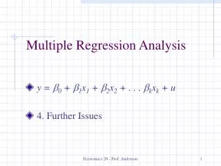
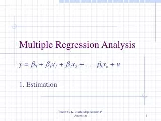
The Model and Assumptions • The multiple regression model is • where yi is the dependent variable for the ith observation • 0 is the Y intercept • 1,.. ,k are the population partial regression coefficients • x1i, x2i,…xkiare the observed values of the independent variables,X1, X2….Xk. • k = 1,2,3…K explanatory variables

The Model and Assumptions • The assumptions of the model are the same as those discussed for simple regression • The expected value of Y for the given Xs is a linear function of the Xs • The standard deviation of the Y terms for given X values is a constant, designated as y|x • The observations, yi, are statistically independent • The distribution of the Y values (error terms) is normal

Interpreting the Partial Regression Coefficients • For each X term there is a partial regression coefficient, k • This coefficient measures the change in the E(Y) given a one unit change in the explanatory variable Xk, • holding the remaining explanatory variables constant • controlling for the remaining explanatory variables • ceteris parabis • Equivalent to a partial derivative in calculus

Method of Least Squares - OLS • To estimate the population regression equation, we use the method of least squares • The model written in terms of the sample notation is • The sample regression equation is

Method of Least Squares - OLS • Goal is to minimize the distance between the predicted values of Y, the , and the observed values, yi, that is, minimize the residual, ei • Minimize

Method of Least Squares - OLS • Take partial derivatives of SSE with respect to each of the partial regression coefficients and the intercept • Each equation is set equal to zero • This gives us k+1 equations in k+1 unknowns • The equations must be independent and non-homogeneous • Using matrix algebra or a computer, this system of equations can be solved • With a single explanatory variable, the fitted model is a straight line • With two explanatory variables, the model represents a plane in a three dimensional space • With three or more variables it becomes a hyperplane in higher dimensional space • The sample regression equation is correctly called a regression surface, but we will call it a regression line

An Example: The Human Capital Model • Consider education as an investment in human capital • There should be a return on this investment in terms of higher future earnings • Most people accept that earnings tend to rise with schooling levels, but this knowledge by itself does not imply that individuals should go on for more schooling • More is usually costly • Direct payments (tuition) • Indirect payments (foregone earnings) • Thus the actual magnitude of the increased earnings with additional years of schooling is important • Can not simply calculate the average earnings for a sample of workers with different education levels • Have to consider the effects on earnings of other factors, for example, experience in the labor market, age, ability, race and sex

An Example: The Human Capital Model • Consider a first simple model • (1) Earnings = 0 + 1education + • Expect that the coefficient on education will be positive, 1 > 0 • Realize that most people have higher earnings as they age, regardless of their education • If age and education are positively correlated, the estimated regression coefficient on education will overstate the marginal impact of education • A better model would account for the effect of age • (2) Earnings =0 + 1education +2age + 

A Conceptual Experiment • Multiple regression involves a conceptual experiment that we might not be able to carry out in practice • What we would like to do is to compare individuals with different education levels who are the same age • We would then be able to see the effects of education on average earnings, while controlling for age

Current Population Survey, White Males, March 1991 What is the affect of an additional year of education? $31,523.24 - 27,970.59 = $3,552.65

A Conceptual Experiment • Frequently we do not have large enough data sets to be able to ask this type of question • Multiple regression analysis allows us to perform the conceptual exercise of comparing individuals with the same age and different education levels, even if the sample contains no such pairs of individuals

Sample Data • Data was obtained for the March 1992 Current Population Survey • The CPS is the source of the official Government statistics on employment and unemployment • A very important secondary purpose is to collect information such as age, sex, race, education, income and previous work experience. • The survey has been conducted monthly for over 50 years • About 57,000 households are interviewed monthly, containing approximately 114,500 persons 15 years and older; based on the civilian non-institutional population • For multiple regression question, sample consists of white male respondents 18-65 years old, who spent at least one week in the labor force in the preceding year and who provided information on wage earnings during the preceding year. • Sample size is 30,040 • Students download Multiple Regression Human Capital Hand-out

Sample Statistics In 1991, the average white male in the sample was 37.5 years old, had 13.0 years of education and earned $27,561.92.

Correlation Matrix • Second, consider the correlation matrix, which shows the simple correlation coefficients for all pairs of variables • There is a small, but positive correlation between education and age • A simple regression of earnings on education will overstate the effect of education because education is positively correlated with age and age has a strong positive effect on earnings

Sb0 = Sb1 = Earnings = 0 + 1education + = Se b0 = b1 =

Is Education a Significant Explanatory Variable? • Use t-test • H0: 1≤ 0 No relationship • H1:1> 0 Positive relationship • t-test statistic = 78.709 and the p-value is 0.000 • Reject the H0: 1≤ 0 • There is a significant positive relationship between education and earnings

Additional Information from the Analysis • For each additional year of schooling, average earnings increase by $2,933.78 • The R2 = .1710 • Find that 17.1% of the variation in earnings across workers is explained by variation in education levels • The standard error of the estimate, Se equals $18,876

Sb0 = Sb1 = Sb2 = Earnings = 0 + 1education +2age +  =Se b0 = b1 = b2 =

Interpret the Coefficients • In terms of this problem • For each additional year of schooling, average earnings increase by $2,759.73, controlling for age • For each additional year of age, average earnings increase by $572.74, controlling for schooling

Prediction • Predict the mean earnings for white male workers who are 30 old and have a college degree • The standard error of the estimate, Se = $17,545 where k = no. of explanatory variables

Assessing the Regression as a Whole • Want to assess the performance of the model as a whole • H0: 1 = 2 = 3 = …= k = 0 • The model has no worth • H1: At least one regression coefficient is not equal to zero • The model has worth • If all the b’s are close to zero, then the SSR will approach zero

Assessing the Regression as a Whole • Test Statistic • where k = the number of explanatory variables • If the null hypothesis is true, the calculated test statistic will be close to zero; if the null hypothesis is false, the F test statistic will be “large”

Assessing the Regression as a Whole • The calculated F test statistic is compared with the critical F to determine whether the null hypothesis should be rejected • If Fk,n-k-1 > F,k,n-k-1 (cv) reject the H0 reject ⍺ cv F

ANOVA Table in Regression P-value SSR SSE Finally note the p-value, written as Significance F, which equals 0.0000. This tells us that we have a zero probability of observing a test statistic as large as 5,949.8 if the null hypothesis is true. The model has worth.

Inferences Concerning the Population Regression Coefficients • Which explanatory variables have coefficients significantly different from zero? • Perform a hypothesis test for each explanatory variable • Essentially the same t-test used for simple regression • Hypotheses • H0: k = 0 • H1: k 0

Inferences Concerning the Population Regression Coefficients • The test statistic is • where K = number of independent variables • The denominator, , is the standard error of the regression coefficient, bk • Take the standard errors of the regression coefficients from the computer output

In our model, there are two explanatory variables There will be two tests about population regression coefficients Test whether Education is a significant variable H0: educ≤ 0 H1: educ > 0 Test whether Age is a significant variable H0: age≤ 0 H1: age> 0 Let ⍺ = 0.01 t,.01 = 2.326 from the t tables Inferences Concerning the Population Regression Coefficients

Test statistic: educ Test statistic: age p-values < 0.01 T-test Reject the null hypothesis, one tail test,  = .01. Find that education is significantly and positively related to earnings. Again, we reject the null hypothesis and conclude that age is significantly and positively related to earnings.

The Coefficient of Determination and the Adjusted R2 • The R2 value is still defined as the ratio of the SSR to the SST • We see that 28.38% of the variation in earnings is explained by variation in education and in age • The simple regression has an R2 = 0.1710 • Appears that adding the new explanatory variable improved the “goodness of fit” • This conclusion can be misleading • As we add new explanatory variables to our model, the R2always increases, even when the new explanatory variables are not significant • The SSE always decreases as more explanatory variables are added • This is a mathematical property and doesn’t depend on the relevance of the additional variables

The Coefficient of Determination and the Adjusted R2 • If we take into account the degrees of freedom SSE/(n-k-1) can increase or decrease • Depending on whether the additional variables are significant explanatory variables or not • Adjust the R2 statistic as follows: • Adjusted R2 can increase if the additional explanatory variables are important • Can decrease if the additional explanatory variables are not significant • When comparing regression models with different numbers of explanatory variables, you should compare the adjusted R2 to decide which is the best model • The adjusted R2 1, but can take on a value less than zero if the model is very poor

Online Homework - Chapter 16 Multiple Regression • CengageNOW sixteenth assignment

Multiple Regression Analysis