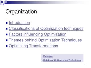
Organization
Organization. Introduction Classifications of Optimization techniques Factors influencing Optimization Themes behind Optimization Techniques Optimizing Transformations. Example Details of Optimization Techniques. Introduction. Concerns with machine-independent code optimization

Organization
E N D
Presentation Transcript
Organization • Introduction • Classifications of Optimization techniques • Factors influencing Optimization • Themes behind Optimization Techniques • Optimizing Transformations • Example • Details of Optimization Techniques
Introduction • Concerns with machine-independent code optimization • 90-10 rule: execution spends 90% time in 10% of the code. • It is moderately easy to achieve 90% optimization. The rest 10% is very difficult. • Identification of the 10% of the code is not possible for a compiler – it is the job of a profiler. • In general, loops are the hot-spots
Introduction • Criterion of code optimization • Must preserve the semantic equivalence of the programs • The algorithm should not be modified • Transformation, on average should speed up the execution of the program • Worth the effort: Intellectual and compilation effort spend on insignificant improvement. Transformations are simple enough to have a good effect
Introduction • Optimization can be done in almost all phases of compilation. Front end Code generator Source code Inter. code target code Profile and optimize (user) Loop, proc calls, addr calculation improvement (compiler) Reg usage, instruction choice, peephole opt (compiler)
Control flow analysis Data flow analysis Transformation Code optimizer Introduction • Organization of an optimizing compiler
Classifications of Optimization techniques • Peephole optimization • Local optimizations • Global Optimizations • Inter-procedural • Intra-procedural • Loop optimization
Factors influencing Optimization • The target machine: machine dependent factors can be parameterized to compiler for fine tuning • Architecture of Target CPU: • Number of CPU registers • RISC vs CISC • Pipeline Architecture • Number of functional units • Machine Architecture • Cache Size and type • Cache/Memory transfer rate
Themes behind Optimization Techniques • Avoid redundancy: something already computed need not be computed again • Smaller code: less work for CPU, cache, and memory! • Less jumps: jumps interfere with code pre-fetch • Code locality: codes executed close together in time is generated close together in memory – increase locality of reference • Extract more information about code: More info – better code generation
Redundancy elimination • Redundancy elimination = determining that two computations are equivalent and eliminating one. • There are several types of redundancy elimination: • Value numbering • Associates symbolic values to computations and identifies expressions that have the same value • Common subexpression elimination • Identifies expressions that have operands with the same name • Constant/Copy propagation • Identifies variables that have constant/copy values and uses the constants/copies in place of the variables. • Partial redundancy elimination • Inserts computations in paths to convert partial redundancy to full redundancy.
Optimizing Transformations • Compile time evaluation • Common sub-expression elimination • Code motion • Strength Reduction • Dead code elimination • Copy propagation • Loop optimization • Induction variables and strength reduction
Compile-Time Evaluation • Expressions whose values can be pre-computed at the compilation time • Two ways: • Constant folding • Constant propagation
Compile-Time Evaluation • Constant folding: Evaluation of an expression with constant operands to replace the expression with single value • Example: area := (22.0/7.0) * r ** 2 area := 3.14286 * r ** 2
Compile-Time Evaluation • Constant Propagation: Replace a variable with constant which has been assigned to it earlier. • Example: pi := 3.14286 area = pi * r ** 2 area = 3.14286 * r ** 2
Constant Propagation • What does it mean? • Given an assignment x = c, where c is a constant, replace later uses of x with uses of c, provided there are no intervening assignments to x. • Similar to copy propagation • Extra feature: It can analyze constant-value conditionals to determine whether a branch should be executed or not. • When is it performed? • Early in the optimization process. • What is the result? • Smaller code • Fewer registers
Common Sub-expression Evaluation • Identify common sub-expression present in different expression, compute once, and use the result in all the places. • The definition of the variables involved should not change Example: a := b * c temp := b * c … a := temp … … x := b * c + 5 x := temp + 5
Common Subexpression Elimination • Local common subexpression elimination • Performed within basic blocks • Algorithm sketch: • Traverse BB from top to bottom • Maintain table of expressions evaluated so far • if any operand of the expression is redefined, remove it from the table • Modify applicable instructions as you go • generate temporary variable, store the expression in it and use the variable next time the expression is encountered. t = a + b x = t ... y = t x = a + b ... y = a + b
Common Subexpression Elimination t1 = a + b c = t1 t2 = m * n d = t2 t3 = b + d e = t3 f = t1 g = -b h = t1 /* commutative */ a = j + a k = t2 j = t3 a = -b if t2 go to L c = a + b d = m * n e = b + d f = a + b g = - b h = b + a a = j + a k = m * n j = b + d a = - b if m * n go to L the table contains quintuples: (pos, opd1, opr, opd2, tmp)
Common Subexpression Elimination • Global common subexpression elimination • Performed on flow graph • Requires available expression information • In addition to finding what expressions are available at the endpoints of basic blocks, we need to know where each of those expressions was most recently evaluated (which block and which position within that block).
Common Sub-expression Evaluation 1 x : = a + b “a + b” is not a common sub-expression in 1 and 4 a : = b 2 3 4 z : = a + b + 10 None of the variable involved should be modified in any path
Code Motion • Moving code from one part of the program to other without modifying the algorithm • Reduce size of the program • Reduce execution frequency of the code subjected to movement
Code Motion • Code Space reduction: Similar to common sub-expression elimination but with the objective to reduce code size. Example: Code hoisting temp : = x ** 2 if (a< b) then if (a< b) then z := x ** 2 z := temp else else y := x ** 2 + 10 y := temp + 10 “x ** 2“ is computed once in both cases, but the code size in the second case reduces.
Code Motion • Execution frequency reduction: reduce execution frequency of partially available expressions (expressions available atleast in one path) Example: if (a<b) then if (a<b) then z = x * 2 temp = x * 2 z = temp else else y = 10 y = 10 temp = x * 2 g = x * 2 g = temp;
Code Motion • Move expression out of a loop if the evaluation does not change inside the loop. Example: while ( i < (max-2) ) … Equivalent to: t := max - 2 while ( i < t ) …
Code Motion • Safety of Code movement Movement of an expression e from a basic block bi to another block bj, is safe if it does not introduce any new occurrence of e along any path. Example: Unsafe code movement temp = x * 2 if (a<b) then if (a<b) then z = x * 2 z = temp else else y = 10 y = 10
Strength Reduction • Replacement of an operator with a less costly one. Example: temp = 5; for i=1 to 10 do for i=1 to 10 do … … x = i * 5 x = temp … … temp = temp + 5 end end • Typical cases of strength reduction occurs in address calculation of array references. • Applies to integer expressions involving induction variables (loop optimization)
Dead Code Elimination • Dead Code are portion of the program which will not be executed in any path of the program. • Can be removed • Examples: • No control flows into a basic block • A variable is dead at a point -> its value is not used anywhere in the program • An assignment is dead -> assignment assigns a value to a dead variable
Dead Code Elimination • Examples: • DEBUG:=0 • if (DEBUG) print Can be • eliminated
Copy Propagation • What does it mean? • Given an assignment x = y, replace later uses of x with uses of y, provided there are no intervening assignments to x or y. • When is it performed? • At any level, but usually early in the optimization process. • What is the result? • Smaller code
Copy Propagation • f := g are called copy statements or copies • Use of g for f, whenever possible after copy statement Example: x[i] = a; x[i] = a; sum = x[i] + a; sum = a + a; • May not appear to be code improvement, but opens up scope for other optimizations.
Local Copy Propagation • Local copy propagation • Performed within basic blocks • Algorithm sketch: • traverse BB from top to bottom • maintain table of copies encountered so far • modify applicable instructions as you go
Loop Optimization • Decrease the number if instruction in the inner loop • Even if we increase no of instructions in the outer loop • Techniques: • Code motion • Induction variable elimination • Strength reduction
Peephole Optimization • Pass over generated code to examine a few instructions, typically 2 to 4 • Redundant instruction Elimination: Use algebraic identities • Flow of control optimization: removal of redundant jumps • Use of machine idioms
Redundant instruction elimination • Redundant load/store: see if an obvious replacement is possible MOV R0, aMOV a, R0 Can eliminate the second instruction without needing any global knowledge of a • Unreachable code: identify code which will never be executed: #define DEBUG 0 if( DEBUG) { if (0 != 1) goto L2 print debugging info print debugging info } L2:
Algebraic identities • Worth recognizing single instructions with a constant operand: A * 1 = A A * 0 = 0 A / 1 = A A * 2 = A + A More delicate with floating-point • Strength reduction: A ^ 2 = A * A
Objective • Why would anyone write X * 1? • Why bother to correct such obvious junk code? • In fact one might write #define MAX_TASKS 1...a = b * MAX_TASKS; • Also, seemingly redundant code can be produced by other optimizations. This is an important effect.
The right shift problem • Arithmetic Right shift: • shift right and use sign bit to fill most significant bits -5 111111...1111111011 SAR 111111...1111111101 which is -3, not -2 • in most languages -5/2 = -2
Addition chains for multiplication • If multiply is very slow (or on a machine with no multiply instruction like the original SPARC), decomposing a constant operand into sum of powers of two can be effective: X * 125 = x * 128 - x*4 + x • two shifts, one subtract and one add, which may be faster than one multiply • Note similarity with efficient exponentiation method
Folding Jumps to Jumps • A jump to an unconditional jump can copy the target address JNE lab1 ...lab1: JMP lab2 Can be replaced by:JNE lab2 As a result, lab1 may become dead (unreferenced)
Jump to Return • A jump to a return can be replaced by a return JMP lab1 ... lab1: RET • Can be replaced byRET lab1 may become dead code
Usage of Machine idioms • Use machine specific hardware instruction which may be less costly. i := i + 1 ADD i, #1 INC i
Optimization of Basic Blocks • Many structure preserving transformations can be implemented by construction of DAGs of basic blocks
DAG representation of Basic Block (BB) • Leaves are labeled with unique identifier (var name or const) • Interior nodes are labeled by an operator symbol • Nodes optionally have a list of labels (identifiers) • Edges relates operands to the operator (interior nodes are operator) • Interior node represents computed value • Identifier in the label are deemed to hold the value
t1 * i 4 t2 + t1, t3 * i 4 Example: DAG for BB t1 := 4 * i t1 := 4 * i t3 := 4 * i t2 := t1 + t3 if (i <= 20)goto L1 (L1) <= 20 i
Construction of DAGs for BB • I/p: Basic block, B • O/p: A DAG for B containing the following information: • A label for each node • For leaves the labels are ids or consts • For interior nodes the labels are operators • For each node a list of attached ids (possible empty list, no consts)
Construction of DAGs for BB • Data structure and functions: • Node: • Label: label of the node • Left: pointer to the left child node • Right: pointer to the right child node • List: list of additional labels (empty for leaves) • Node (id): returns the most recent node created for id. Else return undef • Create(id,l,r): create a node with label id with l as left child and r as right child. l and r are optional params.
Construction of DAGs for BB • Method: For each 3AC, A in B A if of the following forms: • x := y op z • x := op y • x := y • if ((ny = node(y)) == undef) ny = Create (y); if (A == type 1) and ((nz = node(z)) == undef) nz = Create(z);
Construction of DAGs for BB • If (A == type 1) Find a node labelled ‘op’ with left and right as ny and nz respectively [determination of common sub-expression] If (not found) n = Create (op, ny, nz); If (A == type 2) Find a node labelled ‘op’ with a single child as ny If (not found) n = Create (op, ny); If (A == type 3) n = Node (y); • Remove x from Node(x).list Add x in n.list Node(x) = n;
t1 * i 4 Example: DAG construction from BB t1 := 4 * i
[] t2 t1 * i a 4 Example: DAG construction from BB t1 := 4 * i t2 := a [ t1 ]