Physical Oceanography An Introduction
Physical Oceanography An Introduction.

Physical Oceanography An Introduction
E N D
Presentation Transcript
Physical OceanographyAn Introduction • Oceanography is the general name given to the scientific study of the oceans. It is historically divided in terms of the basic sciences into physical, biological, chemical, and geological oceanography. This book is concerned primarily with one of these applications, which is the physics of the ocean. Physical oceanography is historically approached both descriptively and dynamically.
The distinction between these two is often ill-defined, particularly with the recent explosive growth in numerical modeling, which is used for both process modeling and ocean simulation, and assimilation of data into numerical models, mainly for simulation and predictive capability. Perhaps a more useful categorization of scientific approaches is the distinction between those with the goal of understanding a specific process and those with the goal of basic description or simulation of the ocean’s motions. Observations and numerical modeling are used for both of these goals.
The goal of descriptive physical oceanography is to obtain a clear and systematic description of the oceans, sufficiently quantitative to permit us to predict some aspects of their behavior in the future with some certainty. Understanding the basic elements of the ocean environment focuses dynamical understanding and permits useful, quantitative evaluation of ocean models.
Inter-relationships • Generally individual scientists studying the ocean focus on investigations in one of the basic sciences, but very often supporting information may be obtained from observations in other oceanographic disciplines. In fact, one of the intriguing aspects of oceanography is the interdependence of different disciplines.
Why Study Ocean Physics • There are many reasons for developing our knowledge of the oceans. As sources of food, of chemicals and of power, they are as yet only exploited to a minor degree. The oceans provide a vitally important avenue of transportation. They form a sink into which industrial and human waste is dumped, but they do not form a bottomless pit into which material like radioactive waste can be thrown without due thought being given to where it might be carried by currents. The large heat capacity of the oceans exerts a significant and in some cases a controlling effect on the earth’s climate, while the continuous movement of the currents and waves along the coast must be taken into account when piers, breakwaters and other structures are built.
Where does the water go? • In all of these applications, and in many others, knowledge of the ocean circulation is needed. One goal of physical oceanography is to obtain a systematic, quantitative description of the character of the ocean waters, their geographic distribution and of their movements. The latter include the major ocean currents that circulate continuously but with fluctuating velocity and position, medium and small-scale circulation features called the mesoscale features that correspond to weather in the atmosphere, the variable coastal currents, the predictably reversing tidal currents, the rise and fall of the tide, and the waves generated by winds or earthquakes.
Character of the Ocean • The character of the ocean waters includes aspects such as temperature and salt content, which together determine density and hence vertical movement, and also includes other dissolved substances (oxygen, nutrients, chemical species, etc.) or biological species insofar as they yield information about the currents.
Descriptive vs Dynamical • In the descriptive approach to physical oceanography, observations are made of specific features. These are reduced to as simple a statement as possible of the character of the features themselves and of their relations to other features. The dynamical or theoretical approach is to apply the already known laws of physics to the ocean, regarding it as a body acted upon by forces, and to endeavor to solve the resulting mathematical equations to obtain information on the motions to be expected from the forces acting. Numerical modeling is often an adjunct of theoretical physical oceanography; with the goal of understanding well-defined processes with more complex physics than can be treated theoretically.
Observations can be formally combined with such numerical models to improve the simulation and prediction capability. In practice there are limitations and difficulties associated with all of these methods, and our present knowledge of the oceans has been developed by a combination of these approaches. As an example of the combined process, preliminary observations provide some ideas about what features of the ocean require explanation. The basic physical laws that are considered to apply to the situation are then used to set up equations describing the forces acting and the motions observed.
Our present knowledge in physical oceanography represents an accumulation of data, most of which have been gathered during the past 150 years. The purpose of this class is to summarize some of the concepts resulting from studies of these data to give an idea of what we now know about the distribution of the physical characteristics of the ocean waters and of their circulation. We include some of the achievements of dynamical physical oceanography as important context for description. A full treatment of dynamical oceanography is contained in other classes.
History of Physical Oceanography • Physical oceanography has gone through several historical phases. Presumably sailors have always been concerned with ocean currents as they affect their ships’ courses and changes in ocean temperature or surface condition. Many of the earlier navigators, such as Cook and Vancouver, made valuable scientific observations during their voyages in the late 1700s, but it is generally considered that Mathew Fontaine Maury (1855) started the systematic large-scale collection of ocean current data, using ship’s navigation logs as his source of information.
The first major expedition designed expressly to study all the scientific aspects of the oceans was that of the British H.M.S. Challenger which circumnavigated the globe from 1872 to 1876. The first large-scale expedition organized primarily to gather physical oceanographic data was the German FS Meteor expedition to study the Atlantic Ocean from 1925 to 1927. Some of the earliest theoretical studies of the sea were of the surface tides by Newton (1687) and Laplace (1775), and of waves by Gerstner (1847) and Stokes (1874). Following this, about 1896, some of the Scandinavian meteorologists started to turn their attention to the ocean, since dynamical meteorology and dynamical oceanography have much in common. The present basis for dynamical oceanography owes much to the early work of Bjerknes et al (1933), Ekman (1905, 1953), Helland-Hansen (1934) and others.
Subsequent expeditions have added to our knowledge of the oceans, both in single ship and in multi-ship operations including the loosely coordinated worldwide International Geophysical Year projects in 1957—58, the International Indian Ocean Expedition in 1962—65, and the oceanographic aspects of GATE in 1974 (GATE = GARP Atlantic Tropical Experiment where GARP = Global Atmospheric Research Program). In the late 1970s: POLYGON, MODE and POLYMODE in the Atlantic (see Section 7.344), the Coastal Upwelling Ecosystems projects in the Pacific and Atlantic, NORPAX (North Pacific Experiment) and IS0S (International Southern Ocean Study).
In the 1980’s and 1990’s there were two large-scale ocean studies, the World Ocean Circulation Experiment (WOCE) and the Tropical Ocean Global Atmosphere (TOGA) 10-year study (which included the Coupled Ocean Atmosphere Response Experiment = COARE). International programs continuing the study of major interannual, decadal, and much longer variations in climate are being pursued in the late 1990’s and 2000’s, including increasingly global deployment of remote sensing of the oceans, through satellites and telemetering subsurface floats and surface drifters.
Only in a few selected regions do sufficient data exist to allow study of the significant variations in space and time; most of the world’s ocean remains a very sparsely sampled environment. As a result many of today’s research efforts in physical oceanography are focused on developing an understanding of the variability of the ocean as well as a description of its steady state conditions. • More attention has been given in the last few decades than before to the circulation and water properties at the ocean boundaries, along the coasts and in estuaries, and also in the deep and bottom waters of the oceans. Coastal waters are more accessible for observation than the open ocean but show large fluctuations in space and time. Observations have revealed a hitherto unexpected wealth of detail in the form of eddies and shorter-scale time and space variations in the coastal than in the open ocean.
Early Physical Oceanography • The science of physical oceanography has evolved from geographic exploration to the measuring and mapping of real-time changes in the ocean. Early descriptive physical oceanographers were concerned with fundamental descriptions of the oceans, most of which was beneath the surface and which required some ingenuity to sample and describe. An early “data base” for physical oceanography was created by Merz and Wüst of the Meteor Expedition in the 1930’s, consisting of a catalog that recorded each oceanographic station data on a card. Cards could then be combined to study areas or sections of the ocean.
Today’s Descriptive Physical Oceanography • With small data sets, each data point can be considered carefully while statistical analysis is not feasible. Similarly, sparse data sets continue to be collected today, for instance for chemical constituents of seawater, and continue to be analyzed point by point. However, many modern observational techniques generate large volumes of information on currents and water properties. Satellites provide large amounts of data on surface conditions. Within the water column a variety of “floats” provide nearly continuous mapping of currents and temperature.
All of these observations are meshed with increasingly complex numerical simulations of ocean processes. Today’s physical oceanographer may no longer have the luxury of “knowing” each data point and may instead use statistical methods to analyze the large quantities of data now available. Descriptive physical oceanography skills have had to expand to the statistical descriptions of data along with numerical simulations of the ocean environment. Basic familiarity with ocean circulation and water properties remains a necessary foundation.
The ocean and the atmosphere • It will become apparent during our description that there are strong interactions between the ocean and the atmosphere. An example is the El Nino - Southern Oscillation (ENSO) phenomenon which although localized in the tropical Pacific affects climate on time scales of several years over much of the world. To understand such interactions it is necessary to understand the coupled ocean-atmosphere system. In consequence, oceanographers and meteorologists need to work closely together in studying both the hydrosphere and atmosphere and their interactions.
History of Physical Oceanography • The science of oceanography is fairly young. Its origins are in a great variety of earlier studies including some of the earliest applications of physics and mathematics to Earth processes. Some say that Archimedes was one of the earliest physical oceanographers. The familiar Archimedes principle describes the displacement of water by a body placed in the water. Archimedes also made extensive studies of harbors to fortify them against enemy attack.
History of Physical Oceanography • Many early mathematicians also used their skills to study the ocean. Sir Isaac Newton didn’t directly work on problems of the ocean but his principle of universal gravitation was an essential building block in understanding the tides. Both LaPlace and LeGendre put a lot of work into a formal solution of the tides; LaPlace’s equation is a fundamental element in a description of the tides. Other mathematicians worked on a mathematical description of the ocean waves that surrounded their English homeland. All of these studies are clearly part of what we now know as physical oceanography.
Scientists on Ships • One of the earliest applications of physical science to the ocean came from a famous American, Benjamin Franklin. During the many voyages he made between the US and Europe he noticed that some trips were considerably quicker than others. He decided that this was due to a strong ocean current flowing from the west to the east. He had observed some marked changes in surface conditions and reasoned that this ocean current might be marked by a change in sea surface temperature. He began making measurements of the ocean surface temperature during his travels.
Using a simple mercury-in-glass thermometer he was able to determine the position of this current. Working with whaling Captain Folger, Benjamin Franklin published a map showing the current known as the Gulf Stream (Fig 1.1). In this published chart, Franklin depicted the Gulf Stream and advised ship captains to sail at certain latitudes when going east and others when going west. If they found themselves not making much headway on their westward trip they should sail south and try again. This is an excellent concrete example of how physical oceanography really influenced the course of history.
Charles Darwin and the Beagle • Another source of sea-going physical studies of the ocean came from studies made by “naturalists” who went along on British exploring expeditions. One example was Charles Darwin who went along as the ship’s naturalist of the HMS Beagle on a voyage to chart the southeast shore of South America. This journey included many long visits to the South American continent where Darwin formulated many of his ideas about the origin of species. During the cruise he took measurements of physical ocean parameters such as surface temperature and surface salinity.
There were so many naturalists traveling on British vessels in the early 1800’s that the Royal Society in London decided to design a set of uniform measurements. Then Royal Society secretary Robert Hooke was commissioned to develop the suite of instruments that would be carried by all British government ships. One noteworthy device was a system to measure the bottom depth of the deep ocean. It consisted of a wooden ball float attached to an iron weight. The pair was to be dropped from the ship to descend to the ocean floor where the weight would be dropped; the wooden ball would then ascend to the surface where it would be spotted and collected by the ship.
Organized Expeditions • In 1838 the US Congress had the Navy organize and execute the United States Exploring Expedition to collect oceanographic information from all over the world. Many of the backers of this expedition saw it as a potential economic boon but others were more concerned with the scientific promise of the expedition. In 1836, $300,000 had been appropriated for this expedition. As originally conceived the expedition was to be of particular benefit to natural history, including geology, mineralogy, botany, vegetable chemistry, zoology, ichthyology, ornithology and ethnology. Some practical studies such as meteorology and astronomy were also included in the program.
Most of the science was to be done by a civilian science complement; the Navy was to provide the transportation and some help with the sampling. The Navy did not like this arrangement and insisted that a naval officer lead the entire expedition. This responsibility was given to Lieutenant Charles Wilkes who had earned the reputation of being interested in and able to work on scientific problems. At the same time it was widely known that Wilkes was proud and overbearing, with his own ideas on how this expedition should be executed. Most of the scientific positions were filled with naval personnel. Only nine positions were offered to civilians who were subject to all the rules and conditions of behavior applying to the naval staff.
Unlike other later and more significant single-ship expeditions, 6 naval vessels carried out the United States Exploring Expedition. Starting in Norfolk, Virginia, the expedition sailed across the Atlantic to Madeira, recrossed to Rio de Janeiro, then south around Cape Horn and into the Pacific Ocean. By the time the ships had sailed up the west coast of South America to Callao, Peru, storms had put three ships out of commission. What remained of the expedition crossed the Pacific and while the “scientific gentlemen” were busy making collections in New Holland and New Zealand, two ships, the Vinennes and the Porpoise, sailed south into the Antarctic region where Wilkes believed that there was a large land mass behind a barrier of ice.
In the austral summer of 1839-40 Wilkes sailed his ships south until blocked by the northern edge of the pack ice. He then sailed west along the ice barrier and was able to get close enough to see the land. At one point he came within a nautical mile of the coast of “Termination Land” as Wilkes named it. This was the most interesting part of the expedition as far as Wilkes was concerned. His alleged discovery of Antarctica was strongly contested by the British explorer Sir James Clark Ross but it remains as the only well-known benefit of this mission
Matthew Fountaine Maury • During this same period there was an important development in the U.S. A Navy lieutenant, Matthew Fontaine Maury, was seriously injured in a carriage accident and was not able to go to sea for many years. Instead he was put in charge of a fairly obscure Navy office called the Depot of Charts and Instruments (1842 - 1861). This later became the U.S. Naval Observatory. This depot was responsible for the care of the navigation equipment in use at that time. In addition it received and sent out logs to be filled out by the bridge crew ships. Maury soon realized that the growing number of ship logs in his keeping was an important resource that could be used to benefit many.
His first idea was to make use of the estimates of winds and currents from the ships to develop a climatology of the currents and winds along major shipping routes. At first most people were skeptical about the utility of such maps. Luckily one of the clipper ship captains plying the route between the east and west coasts of the US decided to see if he could use these charts to select the best course of travel for his next voyage. He found that this new information made it possible to cut many days off of his regular travel. As the word got around, other clipper ship captains wanted the same information to help to improve their travel times. Soon other route captains were doing the same and Maury’s information became a publication known as “sailing directions.”
It was under Maury’s guidance that a Lt. Baker developed one of the first deep-sea sounding devices. Lt. Baker stuck with the age-old concept of measuring the ocean depth by dropping a line from the surface. The problem had been that in 4,000 m of water the line became too heavy to retrieve from the surface. Lt Baker designed a new metal line whose cross section varied from a very narrow gauge wire at the bottom to a much thicker wire nearer the surface. In addition, Baker followed one aspect of Hooke’s design and dropped the weight at the bottom, again making the system much lighter for retrieval. A later addition was a small corer added to the end of the line to collect a short (few cms) core of the top-layer of sediment.
This device led to the first comprehensive map of bottom topography of the North Atlantic. Unfortunately for Maury, when the civil war broke out he returned to his native south and spent most of the war developing explosive devices to destroy enemy ships and to barricade harbors. An important part of Maury’s legacy is a book, which he wrote in 1985 and which is still in print, the “Physical Geography of the Sea.”
The Challenger Expedition • The first global oceanographic cruise was made on the British ship the HMS Challenger. This three-year (1872-1876) expedition (Fig. 1.2) was driven primarily by the interest of a pair of biologists (William B. Carpenter and Charles Wyville Thomson) in determining whether or not there is marine life in the great depths of the open ocean. Thomson was a Scot educated as a botanist at the University of Edinburgh and in the late 1860’s he was a professor of natural history at Belfast, Ireland. He had been working with his friend Carpenter, a medical doctor, to discover if the contention by another British naturalist (Edward Forbes) that there was no life below 600 m (called the azoic zone) was true or not. Even in the early phase of the Challenger expedition dredges of bottom material from as much as 2,000 m had demonstrated the great variety of life that exists at the ocean bottom. In addition to biological samples this expedition collected a great number of physical measurements of the sea such as sea surface temperature and samples of the min-max temperatures at various depths.
Along with Thomson and Carpenter, the Challenger scientific staff consisted of a naturalist John Murray and a young chemist, John Young Buchanan, both from the University of Edinburgh. The youngest scientist on the staff was twenty-five-year-old German naturalist Rudolf von Willemoës-Suhm who gave up a position at the University of Munich to join the expedition. Henry Nottidge Moseley, another British naturalist who had also studied both medicine and science, joined the expedition after returning from a Government Expedition to Ceylon. Completing the staff was the expedition’s artist and secretary, James John Wild. Much of the visual documentation that we have from the Challenger Expedition came from the able pen of James Wild. The addition of John Murray was fortuitous in that he later saw to the publication of the scientific results of the expedition. Upon return, it was soon found that the Challenger expedition had exhausted the funds available for the publication of the results. Fortunately Murray, who was really a student from the University of Edinburgh, recognized the value of the phosphate formations that dominated Christmas Island. Claiming the island for England, Murray later set up mining operations on the island. The income from this operation was later used to publish the Challenger reports.
Scandinavian contributions and the dynamic method • In the last quarter of the nineteenth century a group of Scandinavian scientists began to investigate the theoretical complexities of the sea in motion. In the late 1870’s, a Swedish chemist, Gustav Ekman, began studying the physical conditions of the Skagerack, part of the waterway connecting the Baltic and the North Sea. Motivated by fisheries problems, Ekman wanted to explain shoals of herring that had suddenly reappeared in the Skagerack after an absence of 70 years.
He discovered that in the Skagerack there are layers of less-saline water from the Baltic “floating” over the deeper, more saline North Sea water. At the same time he found that herring preferred a particular water layer of intermediate salinity. This shelf, or bank water, as it was called, moved in and out of the Inland Sea and with it went the fish. Ekman knew that his results would not be of any use to the fishermen unless the shelf water and the other layers could be mapped. He joined forces with another Swedish chemist, Otto Pettersson, and together they organized a very thorough series of hydrographic investigations. Pettersson was to emerge from this experience as one of the first physical oceanographers. It should be noted that in Swedish “hydrography” translates as “physical oceanography.
Pettersson and Ekman both understood that to obtain a useful picture of the circulation a series of expeditions involving several vessels that could work together at many times throughout each year would have to be organized. This was a new approach to the study of the sea. In the name of fisheries research such a series of research cruises was begun in the early 1890’s. These were some of the first cruises that emphasized the physical parameters of the ocean. For the vertical profiling of the ocean temperature a new device was available. Since 1874, the English firm Negretti and Zambra had manufactured a reversing thermometer that would give accurate temperatures at depth.
Fridtjof Nansen • During this time, another Scandinavian broke new ground in the rush to reach the North Pole. As a young man of 16, Fridtjof Nansen from Norway was the first person to walk across Greenland. This exploring spirit led Nansen to propose a Norwegian effort to reach the North Pole. From his studies of various evidences, Nansen decided that there was a northwestward circulation of ice in the Arctic. Instead of mounting a large attack on the Arctic, Nansen wanted to build a special ship that could withstand the pressures of the sea ice when the ship was frozen into the Arctic pack ice.
He believed that if he could sail as Far East as possible in summer he could then freeze his ship into the pack ice and be carried to the northwest. His plan was to get as close as possible to the North Pole at which time he and a companion would use dog sleds to reach the pole and then return to the ship. Named the Fram (“forward” in Norwegian) this unique ship was too small to carry a large crew. Instead Nansen gathered a group of nine men who would be able to adapt to this unique experience. Always a scientist, Nansen planned a large number of measurements to be made during the Fram’s time in the ice pack.
On March 1895 the Fram reached 84° N about 360 miles from the pole. Nansen believed that this was about as far north as the Fram was likely to get. In the company of Frederik Hjalmar Johansen and a large number of dogs, Nansen left the relative comfort of the Fram and set off to drive the dog sleds to the North Pole. They drove slowly north over drifting ice until they were within 225 miles of their goal, farther north than any person had been before. For three months they had traveled over extremely rough ice, crossing what Nansen referred to as “congealed breakers” and they had lost their way. From their farthest north point they turned south eventually reaching Franz Josef Land where they hoped to encounter a fishing boat in the short summer season. Surviving by eating their dogs, Nansen and Johansen were very fortunate to meet a British expedition led by Frederick Jackson. In the summer of 1896 they sailed home to Oslo aboard the Windward. Meanwhile the Fram drifted further west and south and emerged from the ice pack just north of Spitsbergen. She sailed back to Oslo and arrived just a week after Nansen and Johansen.
One of Nansen’s primary objectives in the Fram Expedition was to form a more complete idea of the circulations of the northern seas. To achieve this the Fram had taken systematic measurements of the temperatures and salinities of the Arctic water. Using one of Pettersson’s insulated water bottles, Nansen had attached a reversing thermometer to sample the temperature and salinity profiles. This arrangement, known as a “Nansen bottle” is still in use today.
The Ekman Spiral • . Working in the Geophysical Institute of the University of Bergen, Norway, Nansen tried to explain the measurements made by the Fram. The hydrographic measurements suggested a very complex connection between the Norwegian and Arctic Seas. The daily position information from the Fram was also of great interest for this study. As a young student, Ekman worked on this problem with Nansen. Both were interested to note that the Fram did not drift in the same direction as the prevailing wind but instead differed from the wind by about 20° - 40° to the right. • Using the measurements made by the Fram along with simple tank models of the Fram, Ekman developed his theory of the wind-driven circulation of the ocean. Published in 1905 as part of the Fram report, Ekman postulated the response of the ocean to a steady wind in a uniform direction. Making some simple assumptions about the turbulent viscosity of the ocean, Ekman could show how the ocean current response to a steady wind must have a surface current 45° to the right of the wind in the Northern Hemisphere. Below that there is a clockwise (NH.) spiral of currents (called the Ekman spiral) down to a depth where the current vanishes.
The Dynamic Method • In spite of these successes with the Fram data, Nansen realized that he could have done much more. This was motivated by the development of the “dynamic method” for estimating geostrophic ocean currents (see chapter 7). Developed also in Bergen, this method made it possible to map currents at every level from a detailed knowledge of the vertical density structure. The Fram’s measurements were not detailed enough to take best advantage of this technique. This theory was furthered developed by Wilhelm Bjerknes, a professor of meteorology at the University of Oslo, who coined the term “geostrophy” from the Greek “geo” for earth and “strophe” meaning turning.
Johan Sandström and Bjorn Helland-Hansen • . The Norwegian Board of Sea Fisheries had invited Helland-Hansen and Nansen, Johan Hjort, to participate in the first cruise of their new research vessel. They were responsible for the collection of hydrographic measurements. A new problem cropped up. In their process of measuring salinity it was necessary to have a “reference sea water” to make the measurement precise, since slightly different methods and procedures were being used. At this time a Danish physicist, Martin Knudsen, was working on a set of hydrographical tables that would clearly define the relationship between temperature, salinity and density. At the 1899 meeting of the International Council for the Exploration of the Sea (ICES), Knudsen had proposed that such tables be published in order to facilitate the standardization of hydrographic work. For this same reason Knudsen suggested that a Standard or Normal water be created and distributed to oceanographic laboratories throughout the world as a standard against which all salinity measurements could be compared. Knudsen then proceeded to set up the Hydrographical Laboratory for ICES in Copenhagen and the standard seawater later became known as “Copenhagen Water.” He also published standard tables called “Knudsen Tables” which displayed the relationships between chlorinity, salinity, densities and temperature.
Nansen and Helland-Hansen’s careful study of the Norwegian Sea made it the most thoroughly studied and best-known body of water in the world. The new method of computing geostrophic currents had played a large role in defining the circulation of the Norwegian Sea. This “dynamic method’ as it was called was slow to spread to other regions. Then in about 1924, a German oceanographer Georg Wüst applied the dynamic method to the flows at different levels through the Straits of Florida. He compared the results to the current profiles collected by a Lieutenant Pillsbury in the same area with a current meter in the 1880’s. The patterns of the currents were essentially the same and confidence in the dynamic method increased. Another test of the dynamic method arose when the International Ice Patrol (IIP) began to compute the circulation of the northwest Atlantic to track the drift of icebergs. Created after the tragic sinking of the Titanic, the IIP was charged with mapping the positions and drifts of icebergs released into Baffin Bay from the glaciers on Elles Island.
The Meteor Expedition • German scientists performed the real test of the dynamic method on the Meteor expedition in the Atlantic. This expedition was conceived of by a German naval officer, Captain Fritz Spiess to create an opportunity for a German navy vessel to visit foreign ports (prohibited by the treaty at the end of World War I) in the capacity of an ocean research vessel. Captain Spiess had served both prior to and during the war as a hydrographer in the German navy. He realized that to be successful he must find a recognized German scientist to be the “father” of the expedition.