A Vector Version of the 6S Radiative Transfer Code for Atmospheric Correction of Satellite Data
400 likes | 1.17k Vues
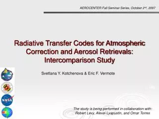
A Vector Version of the 6S Radiative Transfer Code for Atmospheric Correction of Satellite Data. 29 th Review of Atmospheric Transmission Models Meeting Aspects of Polarized Radiative Transfer, June 14. Svetlana Y. Kotchenova & Eric F. Vermote Department of Geography, University of Maryland,

A Vector Version of the 6S Radiative Transfer Code for Atmospheric Correction of Satellite Data
E N D
Presentation Transcript
A Vector Version of the 6S Radiative Transfer Code for Atmospheric Correction of Satellite Data 29th Review of Atmospheric Transmission Models Meeting Aspects of Polarized Radiative Transfer, June 14 Svetlana Y. Kotchenova & Eric F. Vermote Department of Geography, University of Maryland, and NASA GSFC code 614.5
Purpose of the Creation The 6S code is a basic RT code used for the calculation of look-up tables (LUTs) in the MODIS (Moderate Resolution Imaging Spectroradiometer) atmospheric correction (AC) algorithm. Vector 6S LUTs for the AC algorithm AC of MODIS Level 1B data MOD09 (surface reflectance) Movie credit:Blue Marble Project (by R. Stöckli)Reference: R. Stöckli, E. Vermote,N. Saleous, R. Simmon, and D. Herring(2006) "True Color Earth Data Set Includes Seasonal Dynamics", EOS, 87(5), 49-55. www.nasa.gov/vision/earth/features/blue_marble.html different applications 2
History of the Code 1992: development of 5S (Simulation of a Satellite Signal in the Solar Spectrum) byle Laboratoire d’Optique Atmosphérique 1997: development of6S (Second 5S) by Vermote et al. for further use in AC 2004: modification of the scalar 6S to account for polarization by Vermote → 6SV 2005: release of a -version of 6SV by Vermote & Kotchenova → 6SV1.0B 2007: release of version 1.1 of 6SV by Vermote & Kotchenova → 6SV1.1 (SecondSimulation of a Satellite Signal in the Solar Spectrum, Vector, version 1.1) 3
Technical Details RT method: successive orders of scattering Polarization: the Stokes vector {I, Q, U, V= 0} Language: Fortran 77 Input file: Output file: 4
Spectrum: 350 to 3750 nm Molecular atmosphere: 6 code-embedded & 2 user-defined models Instruments: Ground surface: Aerosol atmosphere: homogeneous &non-homogeneous with & without directional effect (10 BRDF + 1 user-defined models) 6 code-embedded & 4 user-defined models & AERONET • AATSR, ALI, ASTER, AVHRR, ETM, GLI, GOES, HRV, HYPBLUE, MAS, MERIS, METEO, MSS, TM, MODIS, POLDER, SeaWiFS, VIIRS, & VGT – 19 in total 6SV Features 5
6SV Accuracy RT simulations: the number of calculation layers and angles default: 30 layers and 48 (Gaussian) angles (accuracy 0.4%) validation work: 50 layers and 148 angles Aerosol simulations: the number of scattering phase function angles default: 83 angles (including 0°, 90°, and 180°) validation work: depends on the case Accuracy-control file: paramdef.inc 6
6SV Validation Effort • The complete 6SV validation effort is summarized in two manuscripts: • S. Y. Kotchenova, E. F. Vermote, R. Matarrese, & F. Klemm, Validation of a vector version of the 6S radiative transfer code for atmospheric correction of satellite data. Part I: Path Radiance, Applied Optics, 45(26), 6726-6774, 2006. • S. Y. Kotchenova & E. F. Vermote, Validation of a vector version of the 6S radiative transfer code for atmospheric correction of satellite data. Part II: Homogeneous Lambertian and anisotropic surfaces, Applied Optics, in press, 2007. testing against benchmarks comparison with other RT codes validation against real measurements resolution of previous 6S accuracy issues 7
Benchmarks (Coulson’s Tables) Coulson’s tabulated values represent the complete solution of the Rayleigh problem for a molecular atmosphere. Standard RT code accuracy requirement: 1% Reference: Muldashev et al., Spherical harmonics method in the problem of radiative transfer in the atmosphere-surface system, Journal of Quantitative Spectroscopy and Radiative Transfer, 61 (3), 393-404, 1999. 8
Benchmarks (Monte Carlo) The code is written by F.M. Bréon (le Laboratoire des Sciences du Climat et de l'Environnement, France) based on the Stokes vector approach. Languages: Fortran, C. Limitations: large amounts of calculation time and angular space discretization. 9
Previous 6S Accuracy Issues Raised in: A. Lyapustin, “Radiative transfer code SHARM-3D for radiance simulations over a non-Lambertian non-homogeneous surface: intercomparison study,” Applied Optics, 41, 5607-5615 (2002). 1. Inability to model aerosols with a highly-asymmetric scattering phase function resolved resolved 2. Incorporation of surface BRDF influence through approximate formulas 10
IKONOS reflectances corrected using AERONET and 6SV vs. reference tarp (portable brightness targets) reflectances Retrieved tarp reflectance Measured tarp reflectance The data were acquired over the Stennis Space Flight Center on February 15, 2002. Experimental Measurements Corrected MODIS Aqua water-leaving reflectances vs. MOBY water-leaving reflectances measured at = {412; 443; 490; 530; 550} nm. The MOBY data were collected off the coast of Lanai Island, Hawaii, during 2003.The analysis is done by R. Matarrese (University of Bari, Italy). 11
Example: The maximum relative error is more than 7%. Effects of Polarization Why is it so important to account for polarization? 12
6SV Web Site http://6S.ltdri.org 13
6SV Interface We provide a special Web interface which can help an inexperienced user learn how to use 6SV and build necessary input files. This interface also lets us track the number and location of 6SV users based on their IP addresses. 14
6SV Users (over the World) Total:898 users 15
6SV Users (Distribution per Country) 6SV e-mail distribution list:145 users 17
available (publiclyor by request) Vector RT Codes Vector RT codes capable of simulating the reflection of solar radiation by a coupled atmosphere-surface system (top-of-atmosphere reflectance): • 6SV • RT3 • Monte Carlo • MODTRAN • VPD ? publicly not available 18
Vector 6S Monte Carlo (benchmark) Dave Vector SHARM (scalar) RT3 Coulson’s tabulated values (benchmark) Code Comparison Project (Description) All information on this project can be found athttp://rtcodes.ltdri.org 19
Code Comparison Project (Rationale) All participating codes are used in different remote sensing applications. 6SV: MODIS atmospheric correction & aerosol retrieval RT3: MODIS aerosol retrieval VPD: TOMS (Total Ozone Mapping Spectrometer) aerosol inversion SHARM: MAIAC (Multi-Angle Implementation of Atmospheric Correction for MODIS) 20
The results will be summarized in a manuscript Project Web site scientific report Code Comparison Project (Goals) • to illustrate the differences between individual simulations of the codes • to determine how the revealed differences influence on the accuracy of atmospheric correction and aerosol retrieval algorithms (Levy et al., Effects of neglecting polarization on the MODIS aerosol retrieval over land, IEEE Transactions on Geoscience and Remote Sensing, 42 (11), 2004 → no effect on aerosol retrieval) • to create a reference (benchmark) data set 21
Code Comparison Project (Results) Molecular atmosphere: done Example: TOA reflectances of the codes vs. Coulson’s tabulated values for τmol = 0.25. Aerosol atmosphere: results are ready for 6SV and SHARM Mixed atmosphere: not done yet 22
Accuracy vs. Speed Example: Time required to simulate TOA reflectance measured by MODIS band 3 over Midway Islands (values in () show how much time is required when the pre-computed aerosol model is read from a file). Computer: Pentium 4 CPU 2.80GHz Reference: Kotchenova & Vermote, 2007 23
6SV Applications • Atmospheric correction (MODIS, VIIRS, etc.) The MODIS data were collected over Alta Foresta on July 16, 2003. MODIS TOA reflectance MODIS surface reflectance • Reference data sets for product validation • Different atmospheric RT simulations 24
Theoretical Error Budget Overall theoretical accuracy of the atmospheric correction method considering the error source on calibration, ancillary data, and aerosol inversion for threeτaer = {0.05 (clear), 0.3 (avg.), 0.5 (hazy)}: Reference: Vermote, E. F. & El Saleous, N. Z. (2006). Operational atmospheric correction of MODIS visible to middle infrared land surface data in the case of an infinite Lambertian target, In: Earth Science Satellite Remote Sensing, Science and Instruments, (eds: Qu. J. et al), vol. 1, chapter 8, 123 - 153. 25
Subsets of Level 1B data processed using the standard surface reflectance algorithm comparison Reference data set AERONET measurements (τaer, H2O, particle distribution) Vector 6S Performance of the MODIS C5 algorithms To evaluate the performance of the MODIS Collection 5 algorithms, we analyzed 1 year of Terra data (2003) over 127 AERONET sites (4988 cases in total). Methodology: If the difference is within ±(0.005+0.05ρ), the observation is “good”. http://mod09val.ltdri.org/cgi-bin/mod09_c005_public_allsites_onecollection.cgi 26
Validation of MOD09 (1) Comparison between the MODIS band 1 surface reflectance and the reference data set. The circle color indicates the % of comparisons within the theoretical MODIS 1-sigma error bar: green > 80%, 65% < yellow <80%, 55% < magenta < 65%, red <55%. The circle radius is proportional to the number of observations. Clicking on a particular site will provide more detailed results for this site. 27
Validation of MOD09 (2) Example: Summary of the results for the Alta Foresta site. Each bar: date & time when coincident MODIS and AERONET observations are available The size of a bar: the % of “good” surface reflectance observations Scatter plot: the retrieved surface reflectances vs. the reference data set along with the linear fit results 28
TOA MOD09-SFC Validation of MOD09 (3) In addition to the plots, the Web site displays a tablesummarizing the AERONET measurementand geometrical conditions, and showsa browse image of the site beforeand after atmospheric correction. Percentage of good: band 1 – 86.62% band 5 – 96.36% band 2 – 94.13% band 6 – 97.69% band 3 – 51.30% band 7 – 98.64% band 4 – 75.18% NDVI – 97.11% EVI– 93.64% Similar results are available for all MODIS surface reflectance products (bands 1-7). 29
Ozone, Stratospheric Aerosols never heard any complaints except from the SHARM developer 20 Km O2, CO2 Trace Gases 8 Km Molecules (Rayleigh Scattering) 2-3 Km H2O, Tropospheric Aerosol Ground Surface Drawbacks 1. Compared to MODTRAN: 6SV Only vertical variation of aerosol profile MODTRAN Vertical variationof aerosol type 2. Compared to SHARM: Speed 30
Future Plans • Non-spherical particlesSolution: combination of 6SV and software for the simulation of non- spherical particles (developed by T. Lapyonok et al. (AERONET group)); preliminary combination work is done by R. Levy (AERONET group). • Polarized surface modelSolution: in process 31
Thanks! Thank you for your attention! Questions:6S@ltdri.org 32