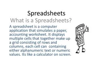
Spreadsheets
Spreadsheets. Unit 1 Charts. Charts. Once you have entered data on a worksheet you can use the Chart wizard to display the data as a chart. You can choose between many different types of charts, four of which are illustrated below:.

Spreadsheets
E N D
Presentation Transcript
Spreadsheets Unit 1 Charts
Charts • Once you have entered data on a worksheet you can use the Chart wizard to display the data as a chart. You can choose between many different types of charts, four of which are illustrated below:
You have control over most aspects of chart construction, including the size, chart title, axis titles and legend. • These chart features are illustrated below.
The chart wizard leads you through the stages required to create a chart. • You can change the appearance of the chart after it has been created by means of the Chart toolbar. • Because the chart is linked to worksheet data, if you change any values that have been used to create the graph the graph is automatically redrawn using the new data.
Create a chart from worksheet data • To create a chart from data in a worksheet: • 1. Select the column or row of figures to be used for the chart. • Include the heading for the figures if there is one.
2. Click the Chart wizard button. The Chart wizard window will appear.
3. Step 1 – Chart type: • Select the type • and form of chart • either from the • Standard types • or Custom types • tab. • 4. Click the • Next button.
Step 2 – Chart source: • Select the range of cells that will be used for the chart. • The correct range of cells to be used should already be set and you should see how the chart will look. • 5. Click the Next button.
Step 3 - Chart options: • Click the Title tab if it not selected and enter the Chart title, Category (X) axis and Value(Y) axis. • 6. Click the Next button.
Step 4 - Chart location: • You can either choose to have the chart embedded in the worksheet containing the data, or you can have the chart drawn in a new worksheet. • 7. Click Finish.
The chart will be displayed in the location chosen in Step 4.
Edit a chart after it has been created • To edit a chart: • 1. Click the right mouse button when the pointer is over the chart.
Chart editing options menu appears. • You will see that there are four options that are the same as steps 1 to 4 of the chart wizard. • 2. Select the chart wizard step required. • You can also click on any of the labels on • the chart (e.g. legend, title) and use the • formatting bar to change the font, font size etc.
Practise creating charts from worksheet data • Visitors to a console games website were asked to vote on the best games console. • The website owners wanted to use this information to judge which console they should concentrate their advertising on for the sale of games.
The results of their survey were as follows: • Console Votes • Atari 1562 • Nintendo 3454 • PlayStation 3122 • Sega 1897 • Xbox 1786 • Others 5341. • Create a worksheet using the above data. • 2. Use the data in the worksheet to produce a bar chart, a column chart and a pie chart. • 3. Experiment with different forms of each of the above types of charts by editing them after you have created them using the chart wizard. • 4. Print an example of each type of chart.