Classical Problem Solving
Classical Problem Solving. Design of Computer Problem Solvers CS 344 Winter 2000. Last time. AI programming versus conventional programming Emphasis on knowledge representation Overview of systems Homework 0 Preview of homework 1. This week’s themes.

Classical Problem Solving
E N D
Presentation Transcript
Classical Problem Solving Design of Computer Problem Solvers CS 344 Winter 2000
Last time • AI programming versus conventional programming • Emphasis on knowledge representation • Overview of systems • Homework 0 • Preview of homework 1
This week’s themes • Problem-solvers see the world in terms of problem spaces • Describe the problem in its own terms, and let Lisp make up the difference
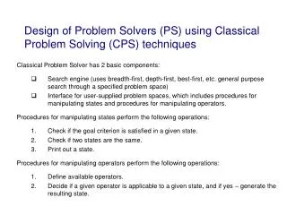
Components of a Problem Space • States (conditions of the world) • Initial state (where we are) • Goal state (where we want to be) • Operators (actions that can change the current state) • Problem solving • Construct a path of states, using available operators, from initial to goal state Problem-solvers see the world in terms of problem spaces
Sample Problem Spaces • Subway travel • Initial state: Davis Street • Goal state: Morse Street • Operators: Take purple line, take red line • Chess • Initial state: Board setup • Goal state: Checkmate condition • Operators: Chess moves Problem-solvers see the world in terms of problem spaces
How to characterize a problem space • Characterizing states • Often symbols or propositional expressions • Comparing states • Choosing operators • Operator applicability (can we use it?) • Operator preference (is it the best one?) • Search strategy • When do we backtrack? Breadth or depth-first? Use means-end analysis? Problem-solvers see the world in terms of problem spaces
Methods for choosing operators • When is an operator applicable? • Preconditions • Which applicable operator is best? • First available • May assume that operators written in order of preference (e.g., travel ops ordered by speed) • Random • Choose one--if it doesn’t work out, try other. • Distance metric • Pick a metric that tells us which is best Problem-solvers see the world in terms of problem spaces
Why study the classical method of problem solving? • Historically early method in AI • GPS (Newell & Simon, 1963) • STRIPS (Fikes & Nilsson, 1971) • Descendants still viable: SOAR, Deep Blue • Provides a vocabulary for discussing problem solving • “States”, “operators”, and “problem spaces” Problem-solvers see the world in terms of problem spaces
Classical Problem Solving • Separation between the search method and the problem space • Search method: generic search methods • Problem space: representation of problem as set of states and operators Problem Space Search Engine
Programming Knowledge Reasoning Engine Knowledge of the domain Computer Program Representation of Domain Knowledge How Problem Spaces provide modularity and explicitness Search Engine Problem Space Representation
Basic search methods • Breadth-first • Try all applicable operators before choosing secondary operators • Depth-first • On the operator chosen, continue searching until either goal is reached or search fails • Best-first • Use a distance metric to choose best operator each time
Building CPS • Need a problem space “API” between a problem space and the search engine • Requirements: • Way to describe basic characteristics of states and operators in problem space • Should provide multiple, interchangable search engines • Should work with novel problem spaces Describe the problem in its own terms, and let Lisp make up the difference.
Constructing a “pluggable” classical problem solver • What’s a pluggable data structure? • Why build a pluggable problem space obj? • Search engines, to be general, need a consistent API for the problem space • No guarantee that all problem spaces will respect that API • Use a pluggable class, called Problem, which mediates between the two and allow an arbitrary problem space to be used with many different search engines. Describe the problem in its own terms, and let Lisp make up the difference.
Code PROBLEM Defstruct • Each problem object defines a particular problem space • E.g., taking subway from MIT to aquarium • Requires following functions to define problem space: • Goal recognizer • State identicality test • Print states • Applicable operators for given state • Distance function Once we have these, we can create “generic” search engines that will work with any problem space.
Using pluggable function slots Function description: PROBLEM slot: When has goal been found? Return set of applicable operators Are states the same? Remove path from possible paths? Estimate of distance to goal Print state Print solution path segment Goal-recognizer Operator-applier States-identical Path-filter Distance-remaining State-printer Solution-element-printer Code
Code Path object structure • Records a particular solution path in terms of intermediate states and operators • Has links back to the problem space, so that a path struct can be taken and “extended” easily.
State and Operator defstructs? • Where’s the state defstruct? • Where’s the op defstruct? • CPS code doesn’t define them. • Instead • Operator and state data structures are implicit in the comparison functions: • Operator-applier, states-identical?, goal-recognizer, distance-remaining, state-printer Describe the problem in its own terms, and let Lisp make up the difference.
Basic search methods • Breadth-first • Try all applicable operators before choosing secondary operators • Depth-first • On the operator chosen, continue searching until either goal is reached or search fails • Best-first • Use a distance metric to choose best operator each time
Bsolve function (simplified) (defun bsolve (initial &aux curr-path new-paths) “Apply breadth-first search to problem space.” (do ((queue (list (list initial initial)) (append (cdr queue) new-paths))) ((null queue)) (setq curr-path (car queue)) (when (goal-recognized? (car curr-path) (return curr-path)) (setq new-paths (extend-path curr-path))
Extend-path (simplified) (defun extend-path (path &aux new-paths new-path pr) “Extend the given path, and return a list of possible paths+1” (setq pr (path-pr path)) (dolist (op (pr-operators pr) new-paths) (dolist (op-pair (apply-op path op pr)) (setq new-path (make-path (add-to-path path (cdr op-pair) (car op-pair)))) (unless (path-has-loop? new-path) ;avoid loops (unless (and (pr-path-filter pr) (funcall (pr-path-filter pr) new-path)) (push new-path new-paths))))))
Extend-path (simplified) (defun extend-path (path &aux new-paths new-path pr) “Extend the given path, and return a list of possible paths+1” (setq pr (path-pr path)) (dolist (op (pr-operators pr) new-paths) (dolist (op-pair (apply-op path op pr)) (setq new-path (make-path (add-to-path path (cdr op-pair) (car op-pair)))) (unless (path-has-loop? new-path) ;avoid loops (unless (and (pr-path-filter pr) (funcall (pr-path-filter pr) new-path)) (push new-path new-paths)))))) Apply each op to path’s end state.
Extend-path (simplified) (defun extend-path (path &aux new-paths new-path pr) “Extend the given path, and return a list of possible paths+1” (setq pr (path-pr path)) (dolist (op (pr-operators pr) new-paths) (dolist (op-pair (apply-op path op pr)) (setq new-path (make-path (add-to-path path (cdr op-pair) (car op-pair)))) (unless (path-has-loop? new-path) ;avoid loops (unless (and (pr-path-filter pr) (funcall (pr-path-filter pr) new-path)) (push new-path new-paths)))))) Apply domain-specific filter.
Bsolve function (simplified) (defun bsolve (initial &aux curr-path new-paths) “Apply breadth-first search to problem space.” (do ((queue (list (list initial initial)) (append (cdr queue) new-paths))) ((null queue)) (setq curr-path (car queue)) (when (goal-recognized? (car curr-path) (return curr-path)) (setq new-paths (extend-path curr-path))
Bsolve function (simplified) Fifo queue (defun bsolve (initial &aux curr-path new-paths) “Apply breadth-first search to problem space.” (do ((queue (list (list initial initial)) (append (cdr queue) new-paths))) ((null queue)) (setq curr-path (car queue)) (when (goal-recognized? (car curr-path) (return curr-path)) (setq new-paths (extend-path curr-path))
Code Bsolve function (simplified) Fifo queue (defun bsolve (initial &aux curr-path new-paths) “Apply breadth-first search to problem space.” (do ((queue (list (list initial initial)) (append (cdr queue) new-paths))) ((null queue)) (setq curr-path (car queue)) (when (goal-recognized? (car curr-path) (return curr-path)) (setq new-paths (extend-path curr-path)) Check current state to see if goal reached:
Bsolve function (simplified) Fifo queue (defun bsolve (initial &aux curr-path new-paths) “Apply breadth-first search to problem space.” (do ((queue (list (list initial initial)) (append (cdr queue) new-paths))) ((null queue)) (setq curr-path (car queue)) (when (goal-recognized? (car curr-path) (return curr-path)) (setq new-paths (extend-path curr-path)) Dsolve LIFO (append new-paths (cdr queue)))
The Agenda type determines the search characteristics FIFO == Breadth-first LIFO == Depth-first
More search variants (variants.lsp) • Best-first search • Estimate distance from goal for each solution path • Sort queue so that closest solution paths tried first • How good must the distance metric be? • Beam search • Same as best-first search, but limit size of queue to a fixed “beam width”
Example 1: Subway navigation Let’s use our search engine to tackle a commonly-used search space: the Boston “T”
Building the representation • Representation • Stations: the lines they are on, x-y map coordinates • Lines: the stations on that line • Problem space mapping • State = station • Operator: Take the line to another station • Definition mechanism • T definitions Describe the problem in its own terms, and let Lisp make up the difference.
Stations (defstruct (subway-station (:PRINT-FUNCTION subway-station-print-procedure)) "Data structure representating a single subway station." (name nil) ;; Name of station. (lines nil) ;; Subways lines it is on. (coordinates nil)) ;; For advanced CPS versions which use a distance metric. (defun subway-station-print-procedure (pr str ignore) "Print name of station." (declare (ignore ignore)) (format str "<Station ~A>" (subway-station-name pr)))
Defining a station (defvar KENDALL-SQUARE) (setq KENDALL-SQUARE (make-subway-station :name ‘Kendall-square :lines ‘(RED-LINE) :coordinates ‘(1 . 0)) (push ‘Kendall-square (subway-line-stations RED-LINE)) (push ‘Kendall-square *stations*)
Defining a station (defmacro defstation (name lines &optional (x 0) (y 0)) "Define a subway station." `(progn (defvar ,name) (setq ,name (make-subway-station :NAME ',name :LINES ',lines :COORDINATES (cons ,x ,y))) ,@ (mapcar #'(lambda (line) `(push ',name (subway-line-stations ,line))) lines) (push ',name *stations*)))
Defining a station (defvar KENDALL-SQUARE) (setq KENDALL-SQUARE (make-subway-station :name ‘Kendall-square :lines ‘(RED-LINE) :coordinates ‘(1 . 0)) (push ‘Kendall-square (subway-line-stations RED-LINE)) (push ‘Kendall-square *stations*) (defstation Kendall-Square (Red-Line) 1.0 0.0) Describe the problem in its own terms, and let Lisp make up the difference.
Defining a station (defstation South-Station (Red-Line) 3.0 -1.0) (defstation Washington (Red-Line Orange-Line) 2.75 -0.75) (defstation Kendall-Square (Red-Line) 1.0 0.0) (defstation Central-Square (Red-Line) -1.0 0.0) (defstation Harvard-Square (Red-Line) -2.0 1.0) (defline Red-Line) (defline Green-Line) (defline Orange-Line) (defline Blue-Line) Describe the problem in its own terms, and let Lisp make up the difference.
Setting up Subway problem PROBLEM: ? ? ? ? ? ? ? Goal-recognizer Operator-applier States-identical Path-filter Distance-remaining State-printer Solution-element-printer
Setting up Subway problem PROBLEM: Subway-states-identical? Subway-operator-finder Subway-states-identical? Prune-subway-path Subway-distance Format Print-subway-path Goal-recognizer Operator-applier States-identical Path-filter Distance-remaining State-printer Solution-element-printer RUN
Next time: Algebra! Brady’s example: log (x+1) + log(x-1) = c.
Classical Problem Solving, II Design of Computer Problem Solvers CS 344 Winter 2000
Lessons from last time • Constructing problem spaces • See a problem in terms of a problem space • How to construct a “pluggable” problem space • Represent the problem in its own terms • Search engines • Breadth, Depth, and Best-First • Fitting the representation to the task • DefLine, DefStation.
Today: Solving algebraic expressions • Algebra as a problem space • Alan Bundy’s model for heuristic-based simplification of algebra problems. • Building the system • Representing states and operators • Pattern matching • How to build it • Making canonical expressions • Homework 1 • Preview of homework 2 (Natural Deduction)
A quick example: Bundy’s challenge 1. loge(x+1) + loge (x-1) = c. 2. loge[(x+1) * (x-1)] = c. 3. loge[x2-1] = c. 4. x2-1=ec. 5. x2 = ec +1. 6. x = +/- sqrt(ec + 1).
Algebra as a Problem Space • The problem space is the transformational grammar • States: valid sentences within that grammar • Operators: transformation operators • Solving algebraic expressions • 3X = 5X - 2. What is the value for X? • Significant expert-novice differences • What do expects know that novices don’t?
Standard Lisp expressions forstates... …named functionsfor operators (takeequation, returns transformed equation). Algebra as a Problem Space • States:Algebraic equations • Initial state:Starting equation. • Goal state:Version of equation with X (unknown) on the left. • Operators: Transformations of the equation using various algebraic laws. • Path:Sets of transformations. • Distance metric: ?? Data structures?
Note: There’s a distance metric hiding in here that we can use later... Bundy’s Claim • Experts have control knowledge that lets them avoid many false paths • This knowledge limits the needed search • Transform equations to reduce the depth and frequency of unknown variable. • Each transformation either reduces the number of unknowns, or brings them closer together. • Three kinds of methods: isolation methods, collection methods, and attraction methods. • This is best understood by graphing the equation.
Isolation methods • Reduces the depth of the occurrences of the unknown • Examples • U - W = Y ®U = Y + W • log(U,w) = Y ®U = WY • Assumptions • U contains x, Y & W do not.
= log - = c e - expt 1 expt 1 expt x 2 e c x 2 Isolation methods Reduce the depth of unknowns. 3. loge[x2-1] = c. 4. x2-1=ec. Depth=4. Depth=3.
Collection methods • Reduce the number of occurrences of the unknown • Examples • UW + UY ® U(W+Y) • (U + V)(U - V) ® U2 - V2 • Assumptions • U and V containx, W & Y do not.
= log c * e - - expt 1 + x 2 x 1 x 1 Collection methods Collect together multiple instances of the unknown: 2. loge[(x+1) * (x-1)] = c. 3. loge[x2-1] = c. One less X.