Sequential Pattern Mining
Sequential Pattern Mining. Outline. What is sequence database and sequential pattern mining Methods for sequential pattern mining Constraint-based sequential pattern mining Periodicity analysis for sequence data. Sequence Databases. A sequence database consists of ordered elements or events

Sequential Pattern Mining
E N D
Presentation Transcript
Outline • What is sequence database and sequential pattern mining • Methods for sequential pattern mining • Constraint-based sequential pattern mining • Periodicity analysis for sequence data
Sequence Databases • A sequence database consists of ordered elements or events • Transaction databases vs. sequence databases A transaction database A sequence database
Applications • Applications of sequential pattern mining • Customer shopping sequences: • First buy computer, then CD-ROM, and then digital camera, within 3 months. • Medical treatments, natural disasters (e.g., earthquakes), science & eng. processes, stocks and markets, etc. • Telephone calling patterns, Weblog click streams • DNA sequences and gene structures
Subsequence vs. super sequence • A sequence is an ordered list of events, denoted < e1 e2 … el> • Given two sequences α=< a1 a2 … an > and β=< b1 b2 … bm > • α is called a subsequence of β, denoted as α⊆ β, if there exist integers 1≤ j1 < j2 <…< jn ≤m such that a1 ⊆ bj1, a2 ⊆ bj2,…, an ⊆ bjn • β is a super sequence of α • E.g.α=< (ab), d> and β=< (abc), (de)>
What Is Sequential Pattern Mining? • Given a set of sequences and support threshold, find the complete set of frequent subsequences A sequence : < (ef) (ab) (df) c b > A sequence database An element may contain a set of items. Items within an element are unordered and we list them alphabetically. <a(bc)dc> is a subsequence of <a(abc)(ac)d(cf)> Given support thresholdmin_sup =2, <(ab)c> is a sequential pattern
Challenges on Sequential Pattern Mining • A huge number of possible sequential patterns are hidden in databases • A mining algorithm should • find the complete set of patterns, when possible, satisfying the minimum support (frequency) threshold • be highly efficient, scalable, involving only a small number of database scans • be able to incorporate various kinds of user-specific constraints
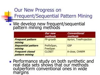
Studies on Sequential Pattern Mining • Concept introduction and an initial Apriori-like algorithm • Agrawal & Srikant. Mining sequential patterns, [ICDE’95] • Apriori-based method: GSP (Generalized Sequential Patterns: Srikant & Agrawal [EDBT’96]) • Pattern-growth methods: FreeSpan & PrefixSpan (Han et al.KDD’00; Pei, et al. [ICDE’01]) • Vertical format-based mining: SPADE (Zaki [Machine Leanining’00]) • Constraint-based sequential pattern mining (SPIRIT: Garofalakis, Rastogi, Shim [VLDB’99]; Pei, Han, Wang [CIKM’02]) • Mining closed sequential patterns: CloSpan (Yan, Han & Afshar [SDM’03])
Methods for sequential pattern mining • Apriori-based Approaches • GSP • SPADE • Pattern-Growth-based Approaches • FreeSpan • PrefixSpan
Seq. ID Sequence 10 <(bd)cb(ac)> 20 <(bf)(ce)b(fg)> 30 <(ah)(bf)abf> 40 <(be)(ce)d> 50 <a(bd)bcb(ade)> The Apriori Property of Sequential Patterns • A basic property: Apriori (Agrawal & Sirkant’94) • If a sequence S is not frequent, then none of the super-sequences of S is frequent • E.g, <hb> is infrequent so do <hab> and <(ah)b> Given support thresholdmin_sup =2
GSP—Generalized Sequential Pattern Mining • GSP (Generalized Sequential Pattern) mining algorithm • Outline of the method • Initially, every item in DB is a candidate of length-1 • for each level (i.e., sequences of length-k) do • scan database to collect support count for each candidate sequence • generate candidate length-(k+1) sequences from length-k frequent sequences using Apriori • repeat until no frequent sequence or no candidate can be found • Major strength: Candidate pruning by Apriori
Seq. ID Sequence min_sup =2 10 <(bd)cb(ac)> 20 <(bf)(ce)b(fg)> 30 <(ah)(bf)abf> 40 <(be)(ce)d> 50 <a(bd)bcb(ade)> Finding Length-1 Sequential Patterns • Initial candidates: • <a>, <b>, <c>, <d>, <e>, <f>, <g>, <h> • Scan database once, count support for candidates
Generating Length-2 Candidates 51 length-2 Candidates Without Apriori property, 8*8+8*7/2=92 candidates Apriori prunes 44.57% candidates
Finding Lenth-2 Sequential Patterns • Scan database one more time, collect support count for each length-2 candidate • There are 19 length-2 candidates which pass the minimum support threshold • They are length-2 sequential patterns
Seq. ID Sequence Cand. cannot pass sup. threshold 5th scan: 1 cand. 1 length-5 seq. pat. <(bd)cba> 10 <(bd)cb(ac)> 20 <(bf)(ce)b(fg)> Cand. not in DB at all <abba> <(bd)bc> … 4th scan: 8 cand. 6 length-4 seq. pat. 30 <(ah)(bf)abf> 3rd scan: 46 cand. 19 length-3 seq. pat. 20 cand. not in DB at all <abb> <aab> <aba> <baa><bab> … 40 <(be)(ce)d> 2nd scan: 51 cand. 19 length-2 seq. pat. 10 cand. not in DB at all 50 <a(bd)bcb(ade)> <aa> <ab> … <af> <ba> <bb> … <ff> <(ab)> … <(ef)> 1st scan: 8 cand. 6 length-1 seq. pat. <a> <b> <c> <d> <e> <f> <g> <h> The GSP Mining Process min_sup =2
The GSP Algorithm • Take sequences in form of <x> as length-1 candidates • Scan database once, find F1, the set of length-1 sequential patterns • Let k=1; while Fk is not empty do • Form Ck+1, the set of length-(k+1) candidates from Fk; • If Ck+1 is not empty, scan database once, find Fk+1, the set of length-(k+1) sequential patterns • Let k=k+1;
The GSP Algorithm • Benefits from the Apriori pruning • Reduces search space • Bottlenecks • Scans the database multiple times • Generates a huge set of candidate sequences There is a need for more efficient mining methods
The SPADE Algorithm • SPADE (Sequential PAttern Discovery using Equivalent Class) developed by Zaki 2001 • A vertical format sequential pattern mining method • A sequence database is mapped to a large set of Item: <SID, EID> • Sequential pattern mining is performed by • growing the subsequences (patterns) one item at a time by Apriori candidate generation
Bottlenecks of Candidate Generate-and-test • A huge set of candidates generated. • Especially 2-item candidate sequence. • Multiple Scans of database in mining. • The length of each candidate grows by one at each database scan. • Inefficient for mining long sequential patterns. • A long pattern grow up from short patterns • An exponential number of short candidates
PrefixSpan (Prefix-Projected Sequential Pattern Growth) • PrefixSpan • Projection-based • But only prefix-based projection: less projections and quickly shrinking sequences • J.Pei, J.Han,… PrefixSpan : Mining sequential patterns efficiently by prefix-projected pattern growth. ICDE’01.
Prefix and Suffix (Projection) • <a>, <aa>, <a(ab)> and <a(abc)> are prefixes of sequence <a(abc)(ac)d(cf)> • Given sequence <a(abc)(ac)d(cf)>
Mining Sequential Patterns by Prefix Projections • Step 1: find length-1 sequential patterns • <a>, <b>, <c>, <d>, <e>, <f> • Step 2: divide search space. The complete set of seq. pat. can be partitioned into 6 subsets: • The ones having prefix <a>; • The ones having prefix <b>; • … • The ones having prefix <f>
Finding Seq. Patterns with Prefix <a> • Only need to consider projections w.r.t. <a> • <a>-projected database: <(abc)(ac)d(cf)>, <(_d)c(bc)(ae)>, <(_b)(df)cb>, <(_f)cbc> • Find all the length-2 seq. pat. Having prefix <a>: <aa>, <ab>, <(ab)>, <ac>, <ad>, <af> • Further partition into 6 subsets • Having prefix <aa>; • … • Having prefix <af>
Completeness of PrefixSpan SDB Length-1 sequential patterns <a>, <b>, <c>, <d>, <e>, <f> Having prefix <c>, …, <f> Having prefix <a> Having prefix <b> <a>-projected database <(abc)(ac)d(cf)> <(_d)c(bc)(ae)> <(_b)(df)cb> <(_f)cbc> <b>-projected database … Length-2 sequential patterns <aa>, <ab>, <(ab)>, <ac>, <ad>, <af> … … Having prefix <aa> Having prefix <af> … <aa>-proj. db <af>-proj. db
The Algorithm of PrefixSpan • Input: A sequence database S, and the minimum support threshold min_sup • Output: The complete set of sequential patterns • Method: Call PrefixSpan(<>,0,S) • Subroutine PrefixSpan(α, l, S|α) • Parameters: • α: sequential pattern, • l: the length of α; • S|α: the α-projected database, if α ≠<>; otherwise; the sequence database S
The Algorithm of PrefixSpan(2) • Method 1. Scan S|α once, find the set of frequent items b such that: a) b can be assembled to the last element of α to form a sequential pattern; or b) <b> can be appended to α to form a sequential pattern. 2. For each frequent item b, append it to α to form a sequential pattern α’, and output α’; 3. For each α’, construct α’-projected database S|α’, and call PrefixSpan(α’, l+1, S|α’).
Efficiency of PrefixSpan • No candidate sequence needs to be generated • Projected databases keep shrinking • Major cost of PrefixSpan: constructing projected databases • Can be improved by bi-level projections
Optimization in PrefixSpan • Single level vs. bi-level projection • Bi-level projection with 3-way checking may reduce the number and size of projected databases • Physical projection vs. pseudo-projection • Pseudo-projection may reduce the effort of projection when the projected database fits in main memory • Parallel projection vs. partition projection • Partition projection may avoid the blowup of disk space
Scaling Up by Bi-Level Projection • Partition search space based on length-2 sequential patterns • Only form projected databases and pursue recursive mining over bi-level projected databases
Speed-up by Pseudo-projection • Major cost of PrefixSpan: projection • Postfixes of sequences often appear repeatedly in recursive projected databases • When (projected) database can be held in main memory, use pointers to form projections • Pointer to the sequence • Offset of the postfix s=<a(abc)(ac)d(cf)> <a> s|<a>: ( , 2) <(abc)(ac)d(cf)> <ab> s|<ab>: ( , 4) <(_c)(ac)d(cf)>
Pseudo-Projection vs. Physical Projection • Pseudo-projection avoids physically copying postfixes • Efficient in running time and space when database can be held in main memory • However, it is not efficient when database cannot fit in main memory • Disk-based random accessing is very costly • Suggested Approach: • Integration of physical and pseudo-projection • Swapping to pseudo-projection when the data set fits in memory
CloSpan: Mining Closed Sequential Patterns • A closed sequential patterns: there exists no superpattern s’ such that s’ כ s, and s’ and s have the same support • Motivation: reduces the number of (redundant) patterns but attains the same expressive power • Using Backward Subpattern and Backward Superpattern pruning to prune redundant search space
Constraints for Seq.-Pattern Mining • Item constraint • Find web log patterns only about online-bookstores • Length constraint • Find patterns having at least 20 items • Super pattern constraint • Find super patterns of “PC digital camera” • Aggregate constraint • Find patterns that the average price of items is over $100
More Constraints • Regular expression constraint • Find patterns “starting from Yahoo homepage, search for hotels in Washington DC area” • Yahootravel(WashingtonDC|DC)(hotel|motel|lodging) • Duration constraint • Find patterns about ±24 hours of a shooting • Gap constraint • Find purchasing patterns such that “the gap between each consecutive purchases is less than 1 month”
From Sequential Patterns to Structured Patterns • Sets, sequences, trees, graphs, and other structures • Transaction DB: Sets of items • {{i1, i2, …, im}, …} • Seq. DB: Sequences of sets: • {<{i1, i2}, …, {im,in, ik}>, …} • Sets of Sequences: • {{<i1, i2>, …, <im,in, ik>}, …} • Sets of trees: {t1, t2, …, tn} • Sets of graphs (mining for frequent subgraphs): • {g1, g2, …, gn} • Mining structured patterns in XML documents, bio-chemical structures, etc.
Episodes and Episode Pattern Mining • Other methods for specifying the kinds of patterns • Serial episodes: A B • Parallel episodes: A & B • Regular expressions: (A | B)C*(D E) • Methods for episode pattern mining • Variations of Apriori-like algorithms, e.g., GSP • Database projection-based pattern growth • Similar to the frequent pattern growth without candidate generation
Periodicity Analysis • Periodicity is everywhere: tides, seasons, daily power consumption, etc. • Full periodicity • Every point in time contributes (precisely or approximately) to the periodicity • Partial periodicit: A more general notion • Only some segments contribute to the periodicity • Jim reads NY Times 7:00-7:30 am every week day • Cyclic association rules • Associations which form cycles • Methods • Full periodicity: FFT, other statistical analysis methods • Partial and cyclic periodicity: Variations of Apriori-like mining methods
Summary • Sequential Pattern Mining is useful in many application, e.g. weblog analysis, financial market prediction, BioInformatics, etc. • It is similar to the frequent itemsets mining, but with consideration of ordering. • We have looked at different approaches that are descendants from two popular algorithms in mining frequent itemsets • Candidates Generation: AprioriAll and GSP • Pattern Growth: FreeSpan and PrefixSpan

