The ancestor problem
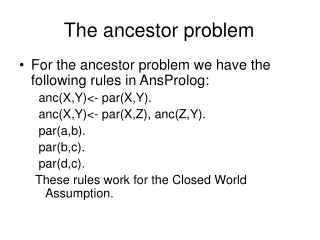
The ancestor problem . For the ancestor problem we have the following rules in AnsProlog: anc(X,Y)<- par(X,Y). anc(X,Y)<- par(X,Z), anc(Z,Y). par(a,b). par(b,c). par(d,c). These rules work for the Closed World Assumption. Ancestor problem (contd.).


The ancestor problem
E N D
Presentation Transcript
The ancestor problem • For the ancestor problem we have the following rules in AnsProlog: anc(X,Y)<- par(X,Y). anc(X,Y)<- par(X,Z), anc(Z,Y). par(a,b). par(b,c). par(d,c). These rules work for the Closed World Assumption.
Ancestor problem (contd.) • Now if our domain consists of the following: par(a,b). par(b,c). ¬par(a,c). ¬par(b,a). then the previous rules work well to find the answers for those that are ancestors. Now consider the problem where we would like to find the set of people who are not ancestors then we have to modify the rules so that we find the set which are not ancestors. We are removing the Closed World Assumption now.
Doing so may involve finding the set of people who may be parents or may not be parents which can be given by: m_par(X,Y)<- not par(X,Y), not ¬par(X,Y). which means that X may or may not be a parent of Y. This rule can be further modified as: m_par(X,Y)<- not ¬par(X,Y). In this case, the classical negation helps us find those X’s who are not parent of Y’s and then the default negation will help us find those X’s who are possibly parent of Y’s. Ancestor problem (contd.)
Ancestor problem (contd.) • So, finally we can get the rule for not ancestors as: m_anc(X,Y)<-m_par(X,Y). m_anc(X,Y)<-m_par(X,Z), m_anc(Z,Y). • This program is mathematically correct for finding the ¬anc(X,Y).
Program Π : anc(X,Y)<-par(X,Y). anc(XY)<-par(X,Z), anc(Z,Y). Let us call this Π and let Π be based on facts D. For example if, Π = par(a,b). ¬par(b,c). Translation of Program Π: m_par(X,Y)<-not ¬par(X,Y). m_anc(X,Y)<-m_par(X,Z), m_anc(Z,Y). Let us call this tr(Π) which means a translation of program Π and it is based on D/ where D/ є ext(D) Π/ = par(a,b). ¬par(b,c). par(b,d). And keep adding to Π/ as long as it remains consistent Correctness of a translation of a program
Correctness of a translation of a program • The complete extension of D would be all the things that are not known to be true or false. • If D/є c_ext(D) (c_ext(D) means a complete extension of D) then tr(Π) U D = for any D/є c_ext(D) • If the conditions are explicitly defined in Π then they should all be reflected to tr(Π). • Automatic translation can be done
Program: fly(X)<-bird(X), not ab(X). bird(tweety). bird(sam). Examples 1. Rules: Birds normally fly. Tweety is a bird. Sam is a bird. If now we add more rules to it we get:
Examples (contd.) 1. Rules: Birds normally fly. Tweety is a bird. Sam is a bird. Penguins are birds. Penguins are exceptional with respect to flying. Sam is a penguin. Now if we wish to find about things that do not fly, we can do that by adding to this program: Program: fly(X)<-bird(X), not ab(X). bird(tweety). bird(sam). (we can strike this out now) bird(X)<-penguin(X). ab(X)<-penguin(X). penguin(sam).
Program now stands: fly(X)<-bird(X), not ab(X). bird(tweety). bird(X)<-penguin(X). ab(X)<-penguin(X). penguin(sam). ¬fly(X)<- not fly(X). ¬bird(X)<- not bird(X). ¬ab(X)<- not ab(X). ¬penguin(X)<- not penguin(X). The last four rules will help us find the objects that do not fly. Examples (contd.)
We further add to our rules: Wounded birds are birds. Wounded birds are weakly exceptional. John is a wounded bird. Note: wounded bird is weakly exceptional, that means that it may or may not fly. The program now adds the following rules: bird(X)<-wounded_bird(X). wounded_bird(john). ab(X)<-wounded_bird(X). ¬fly(X)<- not fly(X), not wounded_bird(X). And removes the rule: ¬fly(X)<- not fly(X). Examples (contd.)
Examples (contd.) The program now stands to: fly(X)<-bird(X), not ab(X). bird(X)<-penguin(X). bird(X)<-wounded_bird(X). ab(X)<-penguin(X). ab(X)<-wounded_bird(X). ¬bird(X)<- not bird(X). ¬ab(X)<- not ab(X). ¬penguin(X)<- not penguin(X). ¬fly(X)<- not fly(X), not wounded_bird(X). bird(tweety). penguin(sam). wounded_bird(john).
Examples (contd.) Adding to the Knowledge base: ¬bird(sylvester). will now help us make the decision that sylvester does not fly by using the rules listed below. fly(X)<-bird(X), not ab(X)……………………….(1) ¬fly(X)<- not fly(X), not wounded_bird(X)…….(2) Sylvester is not a bird and it is not known to be an abnormal bird will make fly(sylvester) false by (1). Again as we have no information about sylvester being wounded and as fly(sylvester) is false by (1) we will infer that sylvester does not fly by (2).
Examples (contd.) Now if we add a constant to the KB et. And we do not know whether et is a bird or not then if we replace the rule ¬fly(X)<- not fly(X), not wounded_bird(X). by ¬fly(X)<- ¬bird(X). Then we reach the conclusion that et does not fly. Also ¬bird(X)<- ¬penguin(X), ¬wounded_bird(X) would lead us to interesting conclusions: as we do not know whether et is a bird or not this rule will give us that et is not a bird as it is not a penguin nor is it a wounded_bird. Thus et does not fly.
Examples (contd.) Thus we have to take care of two important things: • When information are incomplete we have to do certain things • What kind of observations are we allowed to make. So, replacing the ¬bird(X) rule by: ¬bird(X)<- ¬penguin(X), ¬wounded_bird(X), not bird(X). Will in fact give us the correct solution for et. It will give neither et can fly nor et can not fly which is the information that we wish to infer from the KB.
Kinds of Predicates • There are two kinds of predicates: 1. Base Predicates: penguin(X), wounded_bird(X) are base predicates 2. Derived Predicates: These are predicates defined by base predicates. For example, fly(X), bird(X), ab(X) etc. • With incomplete information, what we may want to add to our Knowledge Base may make our derived predicates inconsistent.
Things to remember • When facts are about the base predicates only then adding to KB is straightforward. • If we have classical negation of base predicates then things are fairly simple. • If we allow observation about derived predicates then more advanced techniques are required.
Normally birds fly. Tweety is a bird. Sam is a bird. Sam is a penguin. Wounded birds are birds. Wounded birds are weakly exceptional. i.e., they may fly or may not fly. John is a wounded bird. et. Note: et may or may not be a penguin – we do not know. et is a bird. fly(X)<-bird(X), not ab(X). bird(tweety). bird(et). bird(X)<-penguin(X). bird(X)<-wounded_bird(X). ab(X)<-wounded_bird(X). penguin(sam). ¬penguin(tweety). wounded_bird(john). Then in order to deal with missing data we modify the ab(X) rule as: ab(X)<-not ¬penguin(X). How to handle missing data
Summary • We have to start with normative statements. • Then handle weak exceptions: that is those that are neither known to be true or false. • a) Keeping Close World Assumption in mind like if we know par(X) then the others are not par(X). b) We have to be careful when Close World Assumption is removed. • For new observation, we have to consider what kind of observations can be added so that they do not make the program inconsistent. We have to keep the program consistent. • We have to consider how to assimilate new observation to the Knowledge Base.