Download
1 / 40
410 likes | 845 Vues
4.5 Black-Scholes-Merton Equation part (1). 報告者:顏妤芳. We derive the Black-Scholes-Merton partial differential equation for the price of an option on an asset modeled as a geometric Brownian motion. Determine the initial capital required to perfectly hedge a short position in the option.

E N D
We derive the Black-Scholes-Merton partial differential equation for the price of an option on an asset modeled as a geometric Brownian motion. • Determine the initial capital required to perfectly hedge a short position in the option.
4.5.1 Evolution of Portfolio Value • Consider an agent who at each time t has a portfolio valued at X(t). • This portfolio invests in a money market account paying a constant rate of interest r and in a stock modeled by the geometric Brownian motion (4.5.1) • The investor holds shares of stock. The position can be random but must be adapted to the filtration associated with the Brownian motion W(t),t 0.
MMA = . (4.5.2) • The three terms appearing in the last line of (4.5.2) can be understood as follows: (i) an average underlying rate of return r on the portfolio. (ii) a risk premium for investing in the stock. (iii) a volatility term proportional to the size of the stock investment.
We shall often consider the discounted stock price and the discounted portfolio value of an agent, . According to the It -Doeblin formula with ,the differential of the discounted stock price is (4.5.4)
The differential of the discounted portfolio value is (4.5.5) • Change in the discounted portfolio value is solely due to change in the discounted stock price. 代入(4.5.2)
4.5.2 Evolution of Option Value • Consider a European call option that pays at time T. • We let c(t,x) denote the value of the call at time t if the stock price at that time is S(t)=x. (4.5.6)
We next compute the differential of the discounted option price . Let (4.5.7)
4.5.3 Equating the Evolutions • A (short option) hedging portfolio starts with some initial capital X(0) and invests in the stock and money market account so that the portfolio value X(t) at each time t [0,T] agrees with c(t,S(t)). • One way to ensure this equality is to make sure that (4.5.8) and .
Integration of (4.5.8) from 0 to t then yields (4.5.9) • Comparing (4.5.5) and (4.5.7), • We see that (4.5.8) holds iff (4.5.10)
We first equate the dW(t) terms in (4.5.10), which gives (4.5.11) this is called the delta-hedging rule. • We next equate the dt terms in (4.5.10), obtain = (4.5.12) (4.5.13)
In conclusion, we should seek a continuous function c(t,x) that is a solution to the Black-Scholes-Merton partial differential equation , (4.5.14) • and that satisfies the terminal condition (4.5.15)
So we see that . • Taking the limit as t T and using the fact that both X(t) and c(t,S(t)) are continuous, we conclude that • This means that the short position has been successfully hedged.
4.5.4 solution to the Black-Scholes-Merton Equation • We do not need (4.5.14) to hold at t=T, although we need the function c(t,x) to be continuous at t=T. If the hedge works at all times strictly prior to T, it also works at time T because of continuity. • Equation (4.5.14) is a partial differential equation of the type called backward parabolic. For such an equation, in addition to the terminal condition (4.5.15), one needs boundary conditions at x=0 and x= in order to determine the solution.
The boundary condition at x=0 is obtained by substituting x=0 into (4.5.14), which then becomes (4.5.16) and the solution is Substituting t=T into this equation and using the fact that ,we see that c(0,0)=0 and hence c(t,0)=0 (4.5.17) this is the boundary condition at x=0.
As x ,the function c(t,x) grows without bound. One way to specify a boundary condition at x= for the European call is (4.5.18) • For large x, this call is deep in the money and very likely to end in the money. In this case, the price of the call is almost as much as the price of the forward contract discussed in Subsection 4.5.6 below (see (4.5.26)).
The solution to the Black-Scholes-Merton equation (4.5.14) with terminal condition (4.5.15) and boundary conditions (4.5.17) and (4.5.18) is (4.5.19) Where (4.5.20) and N is the cumulative standard normal distribution (4.5.21)
We shall sometimes use the notation (4.5.22) and call the Black-Scholes-Merton function. • Formula (4.5.19) does not define c(t,x) when t=T,nor dose it define c(t,x) when x=0. • However, (4.5.19) defines c(t,x) in such a way that and
補充 : Dummy Variable • A variable that appears in a calculation only as a placeholder and which disappears completely in the final result.
4.5.5 The Greeks The derivatives of function c( t, x ) of (4.5.19) with respect to various variables are called the Greeks Delta Theta Gamma Vega Rho Psi
The Greeks Delta Gamma Theta
Hedging portfolio At time t, stock price is x, Short a call option The hedging portfolio value is The amount invested in the money market is
Delta-neutral position Because delta and gamma are positive, for fixed t , the function c( t,x ) is increasing and convex in the variable x (see Fig 4.5.1) Consider a portfolio when stock price is we Long a call Short stock Invest in money market account
Option value
Sensitivity to stock price changes of the portfolio The initial portfolio value is zero at time t If the stock price were instantaneously fall to our portfolio value would change to be This is the difference at between the curve and the straight line
Sensitivity to stock price changes of the portfolio Because this difference is positive, our portfolio benefits from an instantaneous drop in the stock price On the other hand, if the stock price were instantaneously rise to It would result the same phenomenon Hence, the portfolio we have set up is said to be delta-neutral and long gamma
Long gamma It benefits from the convexity of c( t,x ) as described above If there is an instantaneously rise or an instantaneously fall in the stock price, the value of the portfolio increases A long gamma portfolio is profitable in times of high stock volatility
Delta-neutral It refers to the fact that the line in Fig 4.5.1 is tangent to the curve When the stock price makes a small move, the change of portfolio value due to the corresponding change in option price is nearly offset by the change in the value of our short position in the stock The straight line is a good approximation to the option price for small stock price moves
Arbitrage opportunity The portfolio described above may at first appear to offer an arbitrage opportunity When we let time move forward both the long gamma position and the positive investment in the money market account offer an opportunity for profit the curve is shifts downward because theta is negative To keep the portfolio delta-neutral, we have to continuously rebalance our portfolio
Vega The derivative of the option price w.r.t. the volatility is called vega The more volatile stocks offer more opportunity from the portfolio that hedges a long call position with a short stock position, and hence the call is more expensive so long as the put option
4.5.6 Put-Call parity A forward contract with delivery price K obligates its holder to buy one share of the stock at the expiration time T in exchange for payment K Let f( t,x ) denote the value of the forward contract at time t, The value of the forward contract at expiration time T
Forward contract Static hedge A hedge that doesn’t trade except at the initial time Consider a portfolio at time 0 Short a forward contract Long a stock Borrow from the money market account
Replicating the payoff of the forward contract At expiration time T of the forward contract Owns a stock S(T) Debt to the money market account grown to K Portfolio value at time T S(T)-K Just replicating the payoff of the forward contract with a portfolio we made at time 0
Forward price The forward price of a stock at time t is defined to be the value of K that cause the forward contract at time t to have value zero i.e., it is the value of K that satisfies the equation The forward price at time t is The forward price isn’t the price of the forward contract
Forward price The forward price at time t is the price one can lock in at time t for the purchase of one share of stock at time T, paying the price at time T Consider a situation at time 0, one can lock in a price for buying a stock at time T Set The value of the forward contract at time t
Put-Call Parity Consider some of the derivatives and their payoff at expiration time T European call European put Forward contract Observe a equation that will hold for any number x (4.5.28)
Put-Call Parity Let x = S(T), the equation (4.5.28) implies The payoff of the forward contract agrees with the payoff of a portfolio that is long a call and short a put The value at time T is holding , so long as holding at all previous times (4.5.29)
Put-Call Parity The relationship of equation (4.5.29) is called put-call parity We can use the put-call parity and the call option formula we derived from the Black-Scholes-Merton formula to obtain the Black-Scholes-Merton put formula