Download
1 / 8
80 likes | 117 Vues
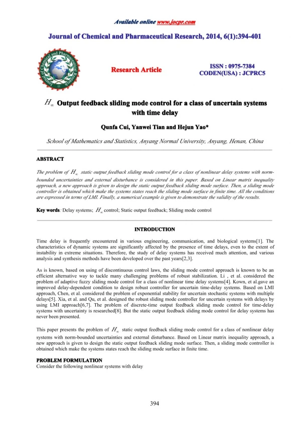
The problem of H∞ static output feedback sliding mode control for a class of nonlinear delay systems with normbounded<br>uncertainties and external disturbance is considered in this paper. Based on Linear matrix inequality<br>approach, a new approach is given to design the static output feedback sliding mode surface. Then, a sliding mode<br>controller is obtained which make the systems states reach the sliding mode surface in finite time. All the conditions<br>are expressed in terms of LMI. Finally, a numerical example is given to demonstrate the validity of the results.

E N D
Available Available Available Available online online online online www.jocpr.com www.jocpr.com www.jocpr.com www.jocpr.com Journal Journal Journal Journal of of of of Chemical Chemical Chemical Chemical and and and and Pharmaceutical Pharmaceutical Pharmaceutical Pharmaceutical Research, Research, Research, Research, 2014, 2014, 2014, 2014, 6(1):394-401 6(1):394-401 6(1):394-401 6(1):394-401 ISSN ISSN ISSN ISSN : : : : 0975-7384 0975-7384 0975-7384 0975-7384 CODEN(USA) CODEN(USA) CODEN(USA) CODEN(USA) : : : : JCPRC5 Research Research Research Research Article Article Article Article JCPRC5 JCPRC5 JCPRC5 H∞Output Output Output Output feedback feedback feedback feedback sliding sliding sliding sliding mode mode mode mode control control control control for with with with with time time time time delay for for for a a a a class delay delay delay class class class of of of of uncertain uncertain uncertain uncertain systems systems systems systems Qunfa Qunfa Qunfa Qunfa Cui, Cui, Cui, Cui, Yanwei Yanwei Yanwei Yanwei Tian Tian Tian Tian and and and and Hejun Hejun Hejun Hejun Yao Yao Yao Yao* * * * School of Mathematics and Statistics, Anyang Normal University, Anyang, Henan, China _____________________________________________________________________________________________ ABSTRACT ABSTRACT ABSTRACT ABSTRACT The problem of H∞static output feedback sliding mode control for a class of nonlinear delay systems with norm- bounded uncertainties and external disturbance is considered in this paper. Based on Linear matrix inequality approach, a new approach is given to design the static output feedback sliding mode surface. Then, a sliding mode controller is obtained which make the systems states reach the sliding mode surface in finite time. All the conditions are expressed in terms of LMI. Finally, a numerical example is given to demonstrate the validity of the results. Key Key Key Key words words words words: Delay systems; H∞control; Static output feedback; Sliding mode control _____________________________________________________________________________________________ INTRODUCTION INTRODUCTION INTRODUCTION INTRODUCTION Time delay is frequently encountered in various engineering, communication, and biological systems[1]. The characteristics of dynamic systems are significantly affected by the presence of time delays, even to the extent of instability in extreme situations. Therefore, the study of delay systems has received much attention, and various analysis and synthesis methods have been developed over the past years[2,3]. As is known, based on using of discontinuous control laws, the sliding mode control approach is known to be an efficient alternative way to tackle many challenging problems of robust stabilization. Li , et al. considered the problem of adaptive fuzzy sliding mode control for a class of nonlinear time delay systems[4]. Kown, et al.gave an improved delay-dependent condition to design robust controller for uncertain time-delay systems. Based on LMI approach, Chen, et al. considered the problem of exponential stability for uncertain stochastic systems with multiple delays[5]. Xia, et al. and Qu, et al. designed the robust sliding mode controller for uncertain systems with delays by using LMI approach[6,7]. The problem of discrete-time output feedback sliding mode control for time-delay systems with uncertainty is researched[8]. But the static output feedback sliding mode control for delay systems has never been presented. This paper presents the problem of H∞static output feedback sliding mode control for a class of nonlinear delay systems with norm-bounded uncertainties and external disturbance. Based on Linear matrix inequality approach, a new approach is given to design the static output feedback sliding mode surface. Then, a sliding mode controller is obtained which make the systems states reach the sliding mode surface in finite time. PROBLEM PROBLEM PROBLEM PROBLEM FORMULATION FORMULATION FORMULATION FORMULATION Consider the following nonlinear systems with delay 394
Hejun Hejun Hejun Hejun Yao ______________________________________________________________________________ ______________________________________________________________________________ ______________________________________________________________________________ ______________________________________________________________________________ Yao Yao Yao et et et et al al al al J. J. J. J. Chem. Chem. Chem. Chem. Pharm. Pharm. Pharm. Pharm. Res., Res., Res., Res., 2014, 2014, 2014, 2014, 6(1):394-401 6(1):394-401 6(1):394-401 6(1):394-401 = = = ( )) ( ) ( A t x t +∆ + ( )) ( A t x t +∆ − + + ωω & ( ) ( ) ( ) x t where ( ) state [ ,0] d − x t y t ( Cx t ψ x t A A d ) Bu t ( ) B ( ) t d d ( ) ( ) t R ∈ delay. A R ∈ (1) − ≤ ≤ d t 0 ∈ ∈ n m p systems output, d is a system initial u t ( ) R y t ( ) given R is system state, systems control input, is R ω ∈ and n n R ∈ are unknown matrices representing the uncertainties and ψ R R ( ) t × the C state on p n × n n × m n × m n × ∈ ∈ ∈ n n R , ( ) A , B R ∆ , ( ) B are known constant matrices, and B has full . d ∈ n n × A t ∆ × d A t column rank. satisfying and ( ) A t ∆ A t ∆ = (2) [ ( )] GD t H ( )[ H ] d d H where , G H and D t is unknown matrix satisfying ( ) are constant matrices with appropriate dimensions, d ≤ T ( ) ( ) D t D t I ω ( ) t is external disturbance and satisfying ω ≤ ρ || ( )|| t ( ) t ρ − where ( ) t is known function on[ d ,0] . U ⎡ ⎤ ⎥ ⎥ ⎦ Ω T ⎡ ⎤ ⎢ ⎥ ⎣ ⎦ B B ω ⎣ [ ] 2 = =⎢ T B U U V T With Singular Value Decomposition of B , , nonsingular transformation is 1 2 0 T U ⎢ ⎣ 1 ⎡ ⎢ ⎣ ⎤ ⎥ ⎦ ⎡ ⎤ ⎥ ⎦ 0 ω 1 = =⎢ constructed for systems(1)to make TB ; TB ω B 2 2 = , the systems(1)can be rewritten With the transformation ( ) z t Tx t ( ) ⎡ ⎢ ⎣ ⎤ ⎥ ⎦ & z t z t & ( ) ( ) 1 = = ( )) ( ) A t x t +∆ + ( )) ( A t x t +∆ − + + ω ( ) z t & T A ( T A ( d ) TBu t ( ) TB ( ) t ω d d 2 − − − − = + ∆ + T A t T + ∆ − 1 1 1 1 ( TAT TBu t + T A t T TB + ( ) ω ) ( ) ( z t TA T ( ) ) ( z t d ) d d ( ) ( ) t ω Inserting (2)into the above formulation, we obtain = + + + + T T T T T z t & ( ) ( + U AU U GDHU z t ) ( ) ( + U AU U GDHU z t ) ( ) ( U A U 1 2 2 2 2 1 2 1 2 1 2 − 2 d 2 − + + + + ωω T T T U GDH U z t + ) ( ) ( d U A U U GDH U z t + ) ( d ) B ( ) t 2 d 2 1 2 + d U AU 1 2 d 1 2 1 (3) = T T T T T z t & ( ) ( + U AU U GDHU z t − ) ( ) ( + U GDHU z t ) ( ) ( U A U 2 1 2 1 2 1 1 1 1 1 2 − 1 d 2 + + ωω T T T U G DH U z t ) ( ) ( d U A U U GDH U z t ) ( d ) B u t ( ) B ( ) t 1 d 2 1 1 d 1 2 d 1 2 2 2 For the systems(3), selecting the static output feedback sliding mode surface as following σ = ( ) t Sy t ( ) (4) 395
Hejun Hejun Hejun Hejun Yao ______________________________________________________________________________ ______________________________________________________________________________ ______________________________________________________________________________ ______________________________________________________________________________ Yao Yao Yao et et et et al al al al J. J. J. J. Chem. Chem. Chem. Chem. Pharm. Pharm. Pharm. Pharm. Res., Res., Res., Res., 2014, 2014, 2014, 2014, 6(1):394-401 6(1):394-401 6(1):394-401 6(1):394-401 With − σ = = = = + = 1 ( ) t Sy t ( ) SCT z t ( ) SC U [ U z t ] ( ) SCU z t ( ) SCU z t ( ) 0 2 1 2 1 1 2 SCU is nonsingular, we obtain by the assumption that 1 − = − = − 1 z t ( ) ( SCU ) SCU z t ( ) Fz t ( ) 2 1 2 1 1 − = 1 F ( SCU ) SCU Where . 1 2 Inserting the above formulation into the systems(3), the sliding mode equation is obtained = + − + ωω z t & ( ) Az t ( ) A z t ( d ) B ( ) t (5) 1 1 d 1 1 where = − + − T T A U A U = ( U F − ) U GDH U + ( U F − ) 2 2 1 U F 2 U GDH U 2 ( 1 T T A U A U ( ) U F ) d 2 d 2 1 2 d 2 1 RESULTS RESULTS RESULTS RESULTS ε > ≤ T 0 F F I D E F which satisfying , , Lemma1 Lemma1 Lemma1 Lemma1[2] For known constant matrix inequality is hold and matrices , then the following ε− + ≤ DD ε + T T T T 1 T DEF E F D E E Lemma2 Lemma2 Lemma2 Lemma2[9]The LMI Y x ⎡ ⎢ ⎣ ⎤> ⎥ ⎦ ( ) * W x R x ( ) ( ) 0 is equivalent to − − > R x > 1 T Y x ( ) W x R ( ) ( ) x W ( ) x 0 ( ) 0 , = = T T depend on x . Y x ( ) Y ( ), ( ) x R x R ( ) x where α > 0 , the sliding mode equation is stable and the H∞performance index of , if there exist positive-definite matrices ,constants 2 3 , ρ ρ and matrices Z Theorem1 Theorem1 Theorem1 Theorem1 For the given constants , , % % − − n m − ) ( × n m − system γ is singular values of % % ∈ 1 T ( ) X RX P Q R R , × n m − ∈ m ( ) N % R n m − ) ( × n m − ∈ ( ) matrices linear matrix inequality holds ⎡ Σ Σ ⎢ ∗ Σ ⎢ ⎢ ∗ ∗ ⎢ ∗ ∗ ⎢ ⎢ ∗ ∗ ⎢ ∗ ∗ ⎢ ⎣ such that the following X N , , N , R 1 2 3 % % % ⎤ ⎥ ⎥ ⎥ ⎥ ⎥ ⎥ ⎥ ⎥ ⎦ Σ Σ Σ − Σ Σ T B X B X B X R − ∗ ∗ dN dN dN ω 11 12 13 1 1 16 − − ρ ρ T ω 22 23 2 1 2 26 0 0 0 α − T < ω 33 ∗ ∗ ∗ 3 1 3 (6) 0 0 dQ − ∗ % I 396
Hejun Hejun Hejun Hejun Yao ______________________________________________________________________________ ______________________________________________________________________________ ______________________________________________________________________________ ______________________________________________________________________________ Yao Yao Yao et et et et al al al al J. J. J. J. Chem. Chem. Chem. Chem. Pharm. Pharm. Pharm. Pharm. Res., Res., Res., Res., 2014, 2014, 2014, 2014, 6(1):394-401 6(1):394-401 6(1):394-401 6(1):394-401 where Σ = Σ = Σ = Σ = Σ Σ Σ Σ N % % N % % + − − − ) ( − − + U GG U α T T T T T T T T U A U X − − ( U Z − − U X ρ − U Z ) A U 11 1 1 2 2 1 2 1 2 2 αρ + 2 − T T T T T T T T N % % N U A U X ( U Z ) ( U X U Z ) A U U GG U 12 2 + 1 + − % 2 d ρ 2 1 2 2 1 2 2 2 2 + U GG U αρ T T T T T T T P N X ( U X U Z ) A U 13 3 3 2 1 2 3 2 2 T T T U X = − = − = = ( U Z ) H 16 2 % 1 − − + ρ − − − ρ − + αρ T T T T T T d 2 2 T T N % N ρ − U A U X ρ ( U Z ) ( U X αρ ρ U Z ) A U U GG U 22 2 2 2 2 d 2 1 2 + 2 1 2 2 2 − T T T T T d T T N X ( U X U Z ) A U U GG U 23 2 1 2 3 2 1 2 2 3 2 2 T T T d ( U X % U Z ) ρ H 26 2 1 + ρ + + αρ T 2 3 T T dQ X X U GG U 33 3 3 2 2 We can Design the sliding mode surface σ = ( ) t Sy t ( ) Where matrix S satisfying ZX− − = = T SC U F ( U ) 0, F 1 2 Proof. Selecting Lyapunov functional such as 0 t +∫ ∫ = θ T T z & ( ) s Qz s dsd & V t ( ) z t Pz t ( ) ( ) ( ) 1 1 1 1 − + θ d t , P Q are positive-definite matrices of Theorem1. Where Then, along the solution of system (5) we have t ( ) & t d − ∫ = + − + T T T T & dz t Qz t & & z & ( ) s Qz s ds & V t 2 z t Pz t ( ) ( ) ( ) ( ) ( ) 2( z t N ( ) 1 1 1 1 1 1 1 1 t t d − ∫ + − + − − − T T z s ds & z t ( d N ) z t N ( ) )( ( ) z t z t ( d ) ( ) ) 1 2 1 3 1 1 1 + + − + − − − + T T T z t M & ∫ ( )) & 2( z t M ( ) z t ( d M ) ( ) )( Az t ( ) A z t ( d ) z t 1 1 1 2 1 3 1 d 1 1 t ≤ + − + + − T T T T T & dz t Qz t & & z & ( ) s Qz s ds & 2 z t Pz t ( ) ( ) ( ) ( ) ( ) 2( z t N ( ) z t ( d N ) 1 1 1 1 1 1 1 1 1 2 t d − + − − − )) 2( d + + & + − + − T T T T z t M & + z t N ( ) )( ( ) z t z t ( z t M ( ) z t + ( d M − ) ( ) )( Az t ( ) 1 3 1 1 1 1 1 2 1 3 1 ( − − − ωω + T T T 1 T A z t ( d ) B ( ) t z t ( )) d z t N ( ( ) z ( t d N ) z t N Q ( ) ) z t N ( ) d 1 1 1 1 1 1 2 1 3 1 1 t t d − ∫ + − + + − γ ω ( ) ( ) t ω + γ ω ( ) ( ) t ω T T T T 2 T 2 T z & ( ) s Qz s ds & z t ( d N ) z t N ( ) ) ( ) t t 1 2 1 3 1 1 = ξ Ξ ξ + γ ω ( ) ( ) t ω T 2 T ( ) t ( ) t t N N N M M M are constant matrices with appropriate dimensions to be confirmed. , , , , , where 1 2 3 1 2 3 397
Hejun Hejun Hejun Hejun Yao ______________________________________________________________________________ ______________________________________________________________________________ ______________________________________________________________________________ ______________________________________________________________________________ Yao Yao Yao et et et et al al al al J. J. J. J. Chem. Chem. Chem. Chem. Pharm. Pharm. Pharm. Pharm. Res., Res., Res., Res., 2014, 2014, 2014, 2014, 6(1):394-401 6(1):394-401 6(1):394-401 6(1):394-401 T ⎡ ⎣ ⎤ ⎦ ξ = − ω T T T T z t & ( ) t z t ( ) z t ( d ) ( ) ( ) t 1 1 1 Ξ Ξ Ξ Ξ Ξ Ξ − − − ⎡ ⎢ ⎢ ⎤ ⎥ ⎥ ⎥ ⎥ ⎦ + M B M B M B γ − ω 11 ∗ ∗ ∗ 12 13 1 1 ω Ξ =⎢ 22 ∗ ∗ 23 2 1 ω 33 ∗ 3 1 ⎢ ⎣ 2 I − Ξ = Ξ = Ξ = Ξ Ξ Ξ + − − − T T T 1 T N N − M A A M − + − dN Q N + 11 1 1 1 1 1 1 − T T T 1 T N N A M M A dN Q N 12 2 + 1 − 2 1 + d dN Q N + 1 2 − T T T 1 T P N − A M − M 13 3 3 1 A M + 1 3 − = − = − = T T d dN Q N T 1 T N N M A + dN Q N 22 2 2 2 d 2 2 2 − − T T d + T 1 T N A M M + 23 3 + 3 2 2 3 − T 1 T dQ M M dN Q N 33 3 3 3 3 The inequality 0 Ξ < (7) is equivalent to ⎡ ⎢ ⎢ ⎢ ⎢ ⎣ ⎤ ⎥ ⎥ ⎥ ⎥ ⎦ ⎡ ⎢ ⎢ ⎢ ⎢ ⎣ ⎡ ⎢ ⎢ ⎢ ⎢ ⎣ ⎤ ⎥ ⎥ ⎥ ⎥ ⎦ T N N N M U G M U G M U G 1 1 2 T [ ⎡ ⎣ ⎤ ⎦ − Ξ = Θ+ − − − 2 1 T T T 2 2 T d Q N N N 0 D H U ( U F ) H U ( U F ) 1 2 3 2 1 d 2 1 3 3 2 0 0 T ⎤ ⎥ ⎥ ⎥ ⎥ ⎦ T M U G M U G M U G 1 2 T ] [ − ] T − − < T 2 2 T 0 0 H U ( U F ) H U ( U F ) 0 0 D 0 2 1 d 2 1 3 2 0 where Θ Θ Θ Θ Θ Θ − − − ⎡ ⎢ ⎢ ⎤ ⎥ ⎥ ⎥ ⎥ ⎦ M B M B M B γ − ω 11 ∗ ∗ ∗ 12 13 1 1 ω Θ =⎢ 22 23 2 1 ∗ ∗ ω 33 3 1 ⎢ ⎣ ∗ 2 I − Θ = + − T T N − N M U A U ( U F ) 11 1 ( 1 U F − 1 2 2 1 T T T Θ = U ) A U M 2 − 1 − 2 1 − T T N − N − M U A U ( U F ) 12 2 U + 1 1 2 d 2 1 T T T Θ = Θ ( U F + ) A U M − 2 N − 1 2 2 − T T T T P M − ( U U F ) A U M 13 3 1 2 1 2 ) 3 = − − = − = − T T N N M U A U ( U F 22 2 2 2 2 d 2 1 − + T T d T Θ Θ ( U U F ) A U M − 2 1 2 U F 2 − T T T d T N M ( U ) A U M 23 3 + 2 + 2 1 2 3 T dQ M M 33 3 3 398
Hejun Hejun Hejun Hejun Yao ______________________________________________________________________________ ______________________________________________________________________________ ______________________________________________________________________________ ______________________________________________________________________________ Yao Yao Yao et et et et al al al al J. J. J. J. Chem. Chem. Chem. Chem. Pharm. Pharm. Pharm. Pharm. Res., Res., Res., Res., 2014, 2014, 2014, 2014, 6(1):394-401 6(1):394-401 6(1):394-401 6(1):394-401 α > With lemma1,we know that the following inequality holds for given constant ⎡ ⎤ ⎢ ⎥ ⎢ ⎥ − − ⎢ ⎥ ⎢ ⎥ ⎣ ⎦ 0 T ⎡ ⎢ ⎢ ⎢ ⎢ ⎣ ⎡ ⎢ ⎢ ⎢ ⎢ ⎣ ⎤ ⎥ ⎥ ⎥ ⎥ ⎦ ⎤ ⎥ ⎥ ⎥ ⎥ ⎦ T T M U G M U G M U G M U G M U G M U G 1 2 T 1 2 T [ ] [ − ] T − − − T 2 2 T 2 2 T D H U ( U F ) H U ( U F ) 0 0 H U ( U F ) H U ( U F ) 0 0 D 2 1 d 2 1 2 1 d 2 1 3 2 3 2 0 0 T ⎡ ⎢ ⎢ ⎢ ⎢ ⎣ ⎤ ⎥ ⎥ ⎥ ⎥ ⎦ T T M U G M U G M U G M U G M U M U G 1 2 T 1 2 T G [ ] [ ] T − ≤ α − − − − + α 1 2 2 T 2 2 T H U ( U F ) H U ( U F ) 0 0 H U ( U F ) H U ( U F ) 0 0 2 1 d 2 1 2 1 d 2 1 3 2 3 2 0 0 With lemma2,we know that the inequality(7)is equivalent to M B M B M B γ ∗ ∗ ∗ − ⎢ ⎢ ∗ ∗ ∗ ∗ ⎢ ∗ ∗ ∗ ∗ ⎣ ( N N M U A U ∆ = + − ∆ = − − ∆ = + + − − ∆ = − ∆ = − − − ∆ = − + − − ∆ = − ∆ = + + + ∆ ∆ ∆ ∆ ∆ ∆ − − − ∆ ∆ ⎡ ⎢ ⎢ ⎢ ⎢ ⎤ ⎥ ⎥ ⎥ ⎥ ⎥ ⎥ ⎥ ⎦ dN dN dN ω 11 ∗ ∗ 12 13 1 1 1 16 ω 22 ∗ 23 2 1 1 26 0 0 0 α − − ω ∆ = < 33 3 1 1 (8) 0 2 I 0 dQ − ∗ ) ( − I U F − + − + M U GG U M α α + T T T T T T T T U F − U ) A U M 11 1 1 1 2 2 1 2 1 2 1 1 2 2 1 ) ( − T T T T T T T T N N M U A U ( U F U U F ) A U M M U GG U M 12 2 1 1 2 U d 2 1 2 1 M U GG U M α 2 2 1 2 2 2 T T T T T T T P N M ( U F ) A U M 13 3 U F 1 2 1 2 3 1 2 2 3 T T ( U ) H 16 2 1 − ) ( − − + M U GG U M α T T T T d T T T T N N M U A U ( U F U α + U F ) A U M 22 2 2 2 2 d 2 1 2 1 2 2 2 2 2 2 T T T d T T T T N M ( U U F ) A U M M U GG U M 23 3 2 2 1 2 3 2 2 2 3 T T d ( U U F ) H 26 2 1 M U GG U M α T T T T dQ M M 33 3 3 3 2 2 3 Pre- and Post-multiplying the inequality (8) by − − − − − − − − − − 1 1 1 1 1 T T T T T diag M { , M , M = , M , M = , } I diag M ρ = { , = M , M , M , M % , } I and , by giving some % 0 0 M 0 M 0 0 ρ 0 X 0 0 0 0 − = = = 1 T T T , M M , M M , M , Z FX , P XPX , Q XQX , transformations 1 0 2 2 0 3 3 0 0 ρ ρ are constants to be obtained, we know that the inequality (8)is equivalent to = γ 2 T , R XX , where 2 3 (6). From the inequality(6), we obtain ( ) & ≤ − ξ Ξ ξ + γ ω ( ) ( ) t ω T 2 T V t ( ) t ( ) t t therefore t t ∫ ∫ − ≤ − ξ ( ) s ds ξ Ξ + γ ω ( ) ( ) s ω T 2 T V t ( ) V t ( ) ( ) s s ds 0 t t 0 0 399
Hejun Hejun Hejun Hejun Yao ______________________________________________________________________________ ______________________________________________________________________________ ______________________________________________________________________________ ______________________________________________________________________________ Yao Yao Yao et et et et al al al al J. J. J. J. Chem. Chem. Chem. Chem. Pharm. Pharm. Pharm. Pharm. Res., Res., Res., Res., 2014, 2014, 2014, 2014, 6(1):394-401 6(1):394-401 6(1):394-401 6(1):394-401 t → ,with the initial condition, we obtain 0 If t t t ∫ ∫ ∫ − λ ( ) Ξ ≤ − λ ( ) Ξ ξ ( ) ( ) s ξ ≤ γ ω ( ) ( ) s ω T T 2 T z ( ) ( ) s z s ds s ds s ds min 1 1 min t t t 0 0 0 Therefore γ ≤ || ( )|| ω || ( )|| z t t . 1 2 2 − λ ( ) Ξ min ( ) & V t < ω = ,we can obtain ,the sliding mode equation is stable. 0 ( ) t 0 If Theorem Theorem Theorem Theorem 2 2 2 2 For the nonlinear delay systems(1),with the controller σ || SC || ( ) t σ t − = − + − + + 1 u t ( ) ( SCB ) [ SCAx t ( ) SCA x t ( d ) (|| GH || || GH || d d (9) || ( )|| + || ( )) ρ + σ + sign ε σ || B t k ( ) t ( )] t ω , k ε are constants satisfying > ε > ,then the systems states will reach the sliding mode surface k 0, 0 Where (4)in finite time. Proof Proof Proof Proof. Along the solution of system (1) we have ( ) ( ) ( ) t t t SC A σ σ σ = & +∆ + σ +∆ − + σ ω T T T T ( ) ( ) A x t ( ) t SC A ( A x t σ ) ( d ) ( ) t SCB ( ) t ω d d || ( ) σ T ( )|| || ( )|| σ ( ) t σ t SC t t − σ − σ − − + T T ( ) t SCAx t ( ) ( ) t SCA x t ( d ) (|| GH || || GH || d d (10) + || ( )) ρ σ − − σ σ σ − σ ε T T || B t ( ) t k ( ) t ( ) t < sign ω ( ) t k ≤ − σ sign ε σ T T With the controller(9)and the above equation(10), we know that the reaching condition is satisfied. ( ) t ( ) t ( ) t 0 CONCLUSION CONCLUSION CONCLUSION CONCLUSION This paper considers the problem of H∞static output feedback sliding mode control for a class of nonlinear delay systems with norm-bounded uncertainties and external disturbance. A static output feedback sliding mode surface is designed by using linear matrix inequality approach. Then the sliding mode controller is designed to make the states reach sliding mode surface in finite time. Acknowledgment Acknowledgment Acknowledgment Acknowledgments s s s The authors would like to thank the associate editor and the anonymous reviewers for their constructive comments and suggestions to improve the quality and the presentation of the paper. This work is supported by National Nature Science Foundation of China under Grant 61073065; Nature Science Foundation of Henan Province under Grant 092300410145; The Education Department of Henan Province Key Foundation under Grant 13A110023. R R R REFERENCES EFERENCES EFERENCES EFERENCES 2002 2002 2002, 46, 219-230. [1]Gouaisbaut F; Dambrine M; Richard J. P. Syst.Contr.Lett., 2002 [2]Kau S. W; Liu Y. S. Syst. Contr. Lett., 2005 [3]Shyu K. K; Liu W. J; Hsu K. C. Automatica, 2005 [4]Li W. L;Yao H. J. Journal of Henan Normal University, 2006 [5]Chen W. H; Guan Z. H; Lu X. M. Syst.Contr.Lett.,2005 [6]Qu S. C; Wang X. Y. Proceeding of the 4th international conference on impulsive and hybrid dynamical systems, 2007 2007 2007 2007,45,1075-1078. [7]Xia Y. Q; Jia Y. M. IEEE Transaction on Automatic Control, 2003 2005 2005 2005,54,1195-1203. 2005 2005 2005, 41, 1239-1246. 2006 2006 2006, 34,14-17. 2005, 54, 547-555. 2005 2005 2003 2003 2003, 48(6),1086-1092. 400
Hejun Hejun Hejun Hejun Yao ______________________________________________________________________________ ______________________________________________________________________________ ______________________________________________________________________________ ______________________________________________________________________________ Yao Yao Yao et et et et al al al al J. J. J. J. Chem. Chem. Chem. Chem. Pharm. Pharm. Pharm. Pharm. Res., Res., Res., Res., 2014, 2014, 2014, 2014, 6(1):394-401 6(1):394-401 6(1):394-401 6(1):394-401 [8]Janardhanan S; Bandyopadhgay B; Thakar V. K. Proceedings of the 2004 IEEE, International Conference on Control Appliactions, 2004 2004 2004 2004, 12, 2-4. [9]Kwon O. M; Park J. H. IEEE Trans. Automatic Control, 2004 2004 2004 2004, 49(11), 14-17. 401