Download
1 / 40

E N D
Comparison of Strategies for Scalable Causal Discovery of Latent Variable Models from Mixed Data Vineet Raghu, Joseph D. Ramsey, Alison Morris, Dimitrios V. Manatakis, Peter Spirtes, Panos K. Chrysanthis, Clark Glymour, and Panayiotis V. Benos
Integrated Biomedical Data Integrated Dataset
Useful Knowledge Requires Causality Patient Stratification Mechanistic Analysis • Without causal understanding of gene-phenotype relationshipswe will not know why treatment plans are working for particular patients • Can lead to problems if these conditions change • Predicting biological mechanismsinherently requires causal knowledge
Properties of this Integrated Dataset • Low sample size • Often in the hundreds • Many variables • ~20,000 genes in the human genome Integrated Dataset Latent confounding • Mixed Data • Continuous expression variables and categorical clinical variables
Today’s Talk • Present new strategies for causal discovery on integrated datasets • Provide a comparison of the benefits of each of the tested approaches on simulated data • Apply one good performing strategy to a real biomedical dataset
Fast Causal Inference (FCI) • Sound and complete algorithm for causal structure learning in the presence of confounding • Five major phases • Adjacency Search (Akin to PC) • Orient Unshielded Colliders • Possible D-SEP to further eliminate adjacencies • Re-Orient colliders with new adjacencies • Make final orientations based on other constraints
Collider Orientation • Orient triple (“A-C-B”) as a collider if C is not in the set that separates A and B • How do we identify the separating set for a pair of variables? B A C
Prior Strategies • FCI and FCI-Stable • Use the smallest separating set found (fewest number of variables) as the true separating set • Conservative FCI (CFCI) • Only orient as a collider if ALL separating sets do not contain the middle variable • Majority Rule FCI • Use all possible separating sets and take majority vote as to whether a collider should be oriented
MAX Strategy • Choose the separating set that has the maximum p-value in its conditional independence test
Constraining the Adjacency Search • Use undirected graph learning method to quickly eliminate unlikely adjacencies • Prevents necessity of full adjacency search • Retains asymptotic correctness iff learned undirected graph is a superset of the true adjacencies
Mixed Graphical Models (MGM) • Pairwise Markov Random Field on mixed variables with the following joint distribution: Continuous-Continuous Edge Potential Source: Lee and Hastie. Learning the Structure of Mixed Graphical Models. 2013. Journal of Computational and Graphical Statistics
Mixed Graphical Models (MGM) • Pairwise Markov Random Field on mixed variables with the following joint distribution: Continuous Node Potential Source: Lee and Hastie. Learning the Structure of Mixed Graphical Models. 2013. Journal of Computational and Graphical Statistics
Mixed Graphical Models (MGM) • Pairwise Markov Random Field on mixed variables with the following joint distribution: Continuous-Discrete Edge Potential Source: Lee and Hastie. Learning the Structure of Mixed Graphical Models. 2013. Journal of Computational and Graphical Statistics
Mixed Graphical Models (MGM) • Pairwise Markov Random Field on mixed variables with the following joint distribution: Discrete-Discrete Edge Potential Source: Lee and Hastie. Learning the Structure of Mixed Graphical Models. 2013. Journal of Computational and Graphical Statistics
MGM Conditional Distributions • Conditional Distribution of Categorical Variables is multinomial • Conditional Distribution of continuous variables is Gaussian
Learning an MGM • Minimize the negative log pseudolikelihood to avoid computing partition function (Proximal Gradient Optimization) • Sparsity penalty employed for each edge type Source: Sedgewick et al. Learning Mixed Graphical Models with Separate Sparsity Parameters and Stability Based Model Selection. 2016. BMC Bioinformatics.
Independence Test (X ⫫ Y | Z) Source: Sedgewick, et al. (2016) Mixed Graphical Models for Causal Analysis of Multimodal Variables. arXiv.
Competitors and Output Metrics • Competitors • FCI-Stable (FCI) • Conservative-FCI (CFCI) • FCI with the MAX Strategy (FCI-MAX) • MGM with the above algorithms • Bayesian Constraint-Based Causal Discovery (BCCD) • Output Metrics • Precision and Recall for PAG Adjacencies and Orientations • Running time of the algorithms
Comparing Partial Ancestral Graphs Comparison of edges only appearing in both the estimated and true graphs
50 Variables, 1000 Samples • Take Away • FCI-MAX improves orientations over all other approaches • BCCD has the best adjacencies on Continuous data, but the FCI approaches perform better with mixed data
50 Variables, 1000 Samples • Take Away • MGM-FCI-MAX provides slight orientation advantage over FCI-MAX alone • Both approaches perform better than MGM-CFCI and MGM-FCI, though these methods can provide better recall
500 Variables, 500 Samples • Take Away • Of the methods that can scale to 500 variables, MFM has the best orientations • FCI maintains an advantage in recall with DD edges but this is parameter dependent
Biomedical Dataset • Goal: Study the effect of HIV on Lung function decline • Variables: Lung function status, smoking history, patient history, demographics and other clinical information for 933 individuals, half with HIV • Filtered low variance variables and samples with missing data for a final dataset of 14 Continuous Variables, 29 Categorical, and 424 samples
Conclusions • MAX strategy improves orientations when balancing precision with recall • Balances orienting too many and not enough colliders • Too slow to be used in practice without optimizations • MGM allows MAX strategy to scale to large numbers of variables on mixed data • Orientations still need to be improved on real data, but adjacencies tend to be highly reliable
Future Directions • More widespread simulation studies with data generated from different underlying distributions to determine useful methods in different situations • Determine accuracy in identifying latent confounders from simulated and real data • Extend this to miRNA-mRNA interactions • Compare parameter selection and stability techniques in the presence of latent variables
Acknowledgements Benos Lab Panagiotis V. Benos and Dimitrios V. Manatakis Panos K. Chrysanthis ADMT Lab University of Pittsburgh Medical Center Alison Morris CMU Department of Philosophy Joseph D. Ramsey, Peter Spirtes, and Clark Glymour
Postdocs wanted! • Develop causal graphical models for integrating biomedical and clinical Big Data • Apply them to cancer and chronic lung diseases Send e-mail to: TakisBenos, PhD Professor and Vice Chair Department of Computational and Systems Biology University of Pittsburgh School of Medicine benos@pitt.edu http://www.benoslab.pitt.edu
Simulating Mixed Data All Continuous X Y Z
Simulating Mixed Data Continuous Child of Mixed Parents X Y Different edge parameter depending upon categorical value of X Z
Simulating Mixed Data Discrete Child Y Z
Simulating Mixed Data Discrete Child Y Z
Bayesian Constraint-Based Causal Discovery (BCCD) Adjacency Search
Bayesian Constraint-Based Causal Discovery (BCCD) Orientations • Orient edges in order of decreasing probability until orientation threshold is reached