Download
1 / 178
1.83k likes | 2.12k Vues
Lecture 03 – Part A Local Search. Dr. Shazzad Hosain Department of EECS North South Universtiy shazzad@northsouth.edu. Beyond IDA* …. So far: systematic exploration: O(b d ) Explore full search space (possibly) using pruning (A*, IDA* … ) Best such algorithms (IDA*) can handle

E N D
Lecture 03 – Part ALocal Search Dr. Shazzad Hosain Department of EECS North South Universtiy shazzad@northsouth.edu
Beyond IDA* … • So far: systematic exploration: O(bd) • Explore full search space (possibly) using pruning (A*, IDA* … ) • Best such algorithms (IDA*) can handle • 10100 states ≈ 500 binary-valued variables • but. . . some real-world problem have 10,000 to 100,000 variables 1030,000 states • We need a completely different approach: • Local Search Methods or Iterative Improvement Methods
Local Search Methods • Applicable when seeking Goal State & don't care how to get there. E.g., • N-queens, • map coloring, • finding shortest/cheapest round trips (TSP) • VLSI layout, planning, scheduling, time-tabling, . . . • resource allocation • protein structure prediction • genome sequence assembly
Local Search Methods Key Idea
Local search • Key idea (surprisingly simple): • Select (random) initial state (generate an initial guess) • Make local modification to improve current state (evaluate current state and move to other states) • Repeat Step 2 until goal state found (or out of time)
Traveling Salesman Person • Find the shortest Tour traversing all cities once.
Traveling Salesman Person • A Solution: Exhaustive Search (Generate and Test) !! The number of all tours is about (n-1)!/2 If n = 36 the number is about: 566573983193072464833325668761600000000 Not Viable Approach !!
Traveling Salesman Person • A Solution: Start from an initial solution and improve using local transformations.
2-opt mutation (2-Swap) for TSP Choose two edges at random
2-opt mutation for TSP Choose two edges at random
2-opt mutation for TSP Remove them
2-opt mutation for TSP Reconnect in a different way (there is only one valid new way) Continue until there is no 2-opt mutation Can be generalized as 3-opt (two valid ways), k-opt etc.
Local Search: Examples N-Queens
Example: 4 Queen • States: 4 queens in 4 columns (256 states) • Operators: move queen in column • Goal test: no attacks • Evaluation: h(n) = number of attacks Not valid initial solution
Local Search: Examples Graph-Coloring
Example: Graph Coloring • Start with random coloring of nodes • Change color of one node to reduce # of conflicts • Repeat 2
Local SearchAlgorithms Basic idea: Local search algorithms operate on a single state – current state – and move to one of its neighboring states. The principle: keep a single "current" state, try to improve it Therefore: Solution path needs not be maintained. Hence, the search is “local”. • Two advantages • Use little memory. • More applicable in searching large/infinite search space. They find reasonable solutions in this case.
Local Search Algorithms Hill Climbing, Simulated Annealing, Tabu Search
Hill Climbing • "Like climbing Everest in thick fog with amnesia" • Hill climbing search algorithm (also known as greedy local search) uses a loop that continually moves in the direction of increasing values (that is uphill). • It teminates when it reaches a peak where no neighbor has a higher value.
evaluation states Hill Climbing
Hill Climbing Initial state … Improve it … using local transformations (perturbations)
Hill Climbing Steepest ascent version function HILL-CLIMBING(problem) returns a solution state inputs: problem, a problem static: current, a node next, a node current MAKE-NODE(INITIAL-STATE[problem]) loop do next a highest-valued successor of current ifVALUE[next] ≤ VALUE[current]then returncurrent current next end
Hill Climbing: Neighborhood Consider the 8-queen problem: • A State contains 8 queens on the board • The neighborhood of a state is all states generated by moving a single queen to another square in the same column (8*7 = 56 next states) • The objective function h(s) = number of pairs of queens that attack each other in state s (directly or indirectly). h(s) = 17 best next is 12 h(s)=1 [local minima]
Hill Climbing Drawbacks • Local maxima/minima : local search can get stuck on a local maximum/minimum and not find the optimal solution Cost Local minimum States
Hill Climbing in Action … Cost States
Hill Climbing Current Solution
Hill Climbing Current Solution
Hill Climbing Current Solution
Hill Climbing Current Solution
Hill Climbing Best Local Minimum Global Minimum
Local Search: State Space A state space landscape is a graph of states associated with their costs
The Goal is to find GLOBAL optimum. How to avoid LOCAL optima? When to stop? Climb downhill? When? Issues
Plateaux A plateu is a flat area of the state-space landscape
Sideways Move • Hoping that plateu is realy a shoulder • Limit the number of sideway moves, otherwise infinite loop • Example: • 100 consecutive sideways moves for 8 queens problem • Chances increase form 14% to 94% • It is incomplete, because stuck at local maxima
Random-restart hillclimbing • Randomly generate an initial state until a goal is found • It is trivially complete with probability approaching to 1 • Example: • For 8-quens problem, very effective • For three million queens, solve the problem within minute
Local Search Algorithms Simulated Annealing (Stochastic hill climbing …)
Simulated Annealing • Key Idea: escape local maxima by allowing some "bad" moves but gradually decrease their frequency • Take some uphill steps to escape the local minimum • Instead of picking the best move, it picks a random move • If the move improves the situation, it is executed. Otherwise, move with some probability less than 1. • Physical analogy with the annealing process: • Allowing liquid to gradually cool until it freezes • The heuristic value is the energy, E • Temperature parameter, T, controls speed of convergence.
SimulatedAnnealing • Basic inspiration: What is annealing? In mettallurgy, annealing is the physical process used to temper or harden metals or glass by heating them to a high temperature and then gradually cooling them, thus allowing the material to coalesce into a low energy cristalline state. Heating then slowly cooling a substance to obtain a strong cristalline structure. • Key idea: Simulated Annealing combines Hill Climbing with a random walk in some way that yields both efficiency and completeness. • Used to solve VLSI layout problems in the early 1980
Simulated Annealing in Action … Cost Best States
Simulated Annealing Cost Best States
Simulated Annealing Cost Best States
Simulated Annealing Cost Best States
Simulated Annealing Cost Best States
Simulated Annealing Cost Best States
Simulated Annealing Cost Best States
Simulated Annealing Cost Best States
Simulated Annealing Cost Best States
Simulated Annealing Cost Best States
Simulated Annealing Cost Best States