Mastering NP-Hardness & Gradient Descent
Learn strategies like Divide and Conquer, Dynamic Programming, and Linear Programming to tackle NP-Hard problems. Explore Vertex Cover, Local Search, Metropolis & Annealing algorithms in detail.


Mastering NP-Hardness & Gradient Descent
E N D
Presentation Transcript
Local Search Instructor: yedeshi yedeshi@gmail.com
Coping With NP-Hardness • What to do if: • Divide and conquer • Dynamic programming • Greedy • Linear Programming/Network Flows • … • does not give a polynomial time algorithm?
Dealing with Hard Problems • Must sacrifice one of three desired features. • Solve problem to optimality. • Solve problem in polynomial time. • Solve arbitrary instances of the problem.
Gradient Descent: Vertex Cover • VERTEX-COVER.Given a graph G = (V, E), find a subset of nodes S of minimal cardinality such that for each u-v in E, either u or v (or both) are in S. • Neighbor relation. S S' if S' can be obtained from S by adding or deleting a single node. Each vertex cover S has at most n neighbors. • Gradient descent. Start with S = V. If there is a neighbor S' that is a vertex cover and has lower cardinality, replace S with S'. • Remark. Algorithm terminates after at most n steps since each update decreases the size of the cover by one.
Gradient Descent: Vertex Cover • Local optimum. No neighbor is strictly better. optimum = all nodes on left side local optimum = all nodes on right side optimum = center node onlylocal optimum = all other nodes optimum = even nodes local optimum = omit every third node
Local Search • Local search. Algorithm that explores the space of possible solutions in sequential fashion, moving from a current solution to a "nearby" one. • Neighbor relation. Let S S' be a neighbor relation for the problem. • Gradient descent. Let S denote current solution. If there is a neighbor S' of S with strictly lower cost, replace S with the neighbor whose cost is as small as possible. Otherwise, terminate the algorithm. A funnel A jagged funnel
Metropolis Algorithm • Metropolis algorithm. [Metropolis, Rosenbluth, Rosenbluth, Teller, Teller 1953] • Simulate behavior of a physical system according to principles of statistical mechanics. • Globally biased toward "downhill" steps, but occasionally makes "uphill" steps to break out of local minima. • Gibbs-Boltzmann function. The probability of finding a physical system in a state with energy E is proportional to e -E/ (kT), where T > 0 is temperature and k is a constant. • For any temperature T > 0, function is monotone decreasing function of energy E. • System more likely to be in a lower energy state than higher one. • T large: high and low energy states have roughly same probability • T small: low energy states are much more probable
Metropolis Algorithm • Metropolis algorithm. • Given a fixed temperature T, maintain current state S. • Randomly perturb current state S to new state S' N(S). • If E(S') E(S), update current state to S'Otherwise, update current state to S' with probability e - E/ (kT), where E = E(S') - E(S) > 0. • Theorem. Let fS(t) be fraction of first t steps in which simulation is in state S. Then, assuming some technical conditions, with probability 1: • Intuition. Simulation spends roughly the right amount of time in each state, according to Gibbs-Boltzmann equation.
Simulated Annealing • Simulated annealing. (Biased towards “downhill”, but also accept “uphill” move) • T large probability of accepting an uphill move is large. • T small uphill moves are almost never accepted. • Idea: turn knob to control T. • Cooling schedule: T = T(i) at iteration i. • Physical analog. • Take solid and raise it to high temperature, we do not expect it to maintain a nice crystal structure. • Take a molten solid and freeze it very abruptly, we do not expect to get a perfect crystal either. • Annealing: cool material gradually from high temperature, allowing it to reach equilibrium at succession of intermediate lower temperatures.
Hopfield Neural Networks • Hopfield networks. Simple model of an associative memory, in which a large collection of units are connected by an underlying network, and neighboring units try to correlate their states. • Input: Graph G = (V, E) with integer edge weights w (positive or negative). • Configuration. Node assignment su= ± 1. • Intuition. If wuv < 0, then u and v want to have the same state;if wuv > 0 then u and v want different states. • Note. In general, no configuration respects all constraints. 7 6 5
Hopfield Neural Networks • Def. With respect to a configuration S, edge e = (u, v) is good if we su sv < 0. • That is, if we < 0 then su = sv; if we > 0, su sv. • Def. With respect to a configuration S, a node u is satisfied if the weight of incident good edges weight of incident bad edges.
Hopfield Neural Networks • Def. A configuration is stable if all nodes are satisfied. • Goal. Find a stable configuration, if such a configuration exists. 4 -1 satisfied node: 5 - 4 - 1 - 1 < 0 -10 -5 -1 bad edge
Hopfield Neural Networks • Goal. Find a stable configuration, if such a configuration exists. • State-flipping algorithm. Repeated flip state of an unsatisfied node. Hopfield-Flip(G, w) { S arbitrary configuration while(current configuration is not stable) { u unsatisfied node su = -su } return S }
State Flipping Algorithm unsatisfied node10 - 8 > 0 unsatisfied node8 - 4 - 1 - 1 > 0 stable
Hopfield Neural Networks • Claim. State-flipping algorithm terminates with a stable configuration after at most W = e|we| iterations. • Pf attempt. Consider measure of progress (S) = # satisfied nodes.
Hopfield Neural Networks • Claim. State-flipping algorithm terminates with a stable configuration after at most W = e|we| iterations. • Pf. Consider measure of progress (S) = e good |we|. • Clearly 0 (S) W. • We show (S) increases by at least 1 after each flip.When u flips state: • all good edges gu incident to u become bad • all bad edges bu incident to u become good • all other edges remain the same u is unsatisfied: bu > gu gu bu
Complexity of Hopfield Neural Network • Hopfield network search problem. Given a weighted graph, find a stable configuration if one exists. • Hopfield network decision problem. Given a weighted graph, does there exist a stable configuration? • Remark. The decision problem is trivially solvable (always yes), but there is no known poly-time algorithm for the search problem. polynomial in n and log W
Maximum Cut • Maximum cut. Given an undirected graph G = (V, E) with positive integer edge weights we, find a node partition (A, B) such that the total weight of edges crossing the cut is maximized.
Applications • Toy application. • n activities, m people. • Each person wants to participate in two of the activities. • Schedule each activity in the morning or afternoon to maximize number of people that can enjoy both activities. • Real applications. Circuit layout, statistical physics.
Maximum Cut • Single-flip neighborhood. Given a partition (A, B), move one node from A to B, or one from B to A if it improves the solution. • Greedy algorithm. Max-Cut-Local (G, w) { Pick a random node partition (A, B) while( improving node v) { if (v is in A) move v to B else move v to A } return (A, B) }
Maximum Cut: Local Search Analysis • Theorem. Let (A, B) be a locally optimal partition and let (A*, B*) be optimal partition. Then w(A, B) ½ e we ½ w(A*, B*). • Pf. Local optimality implies that for all u A : • Adding up all these inequalities yields:
Proof. Con. • Similarly • Now,
Maximum Cut: Big Improvement Flips • Local search. Within a factor of 2 for MAX-CUT, but not poly-time! (Pseudo-poly) • Big-improvement-flip algorithm. Only choose a node which, when flipped, increases the cut value by at least • Claim. Upon termination, big-improvement-flip algorithm returns a cut (A, B) with (2 +)w(A, B) w(A*, B*).
Proof. • Pf. Idea. Add the term to each inequality. • Claim. Big-improvement-flip algorithm terminates after O(-1 n log W) flips, where W = e we. • Each flip improves cut value by at least a factor of (1 + /n). • After n/ iterations the cut value improves by a factor of 2. • Cut value can be doubled at most log W times. if x 1, (1 + 1/x)x 2
Maximum Cut: Context • Theorem. [Sahni-Gonzales 1976] There exists a ½-approximation algorithm for MAX-CUT. • Theorem. [Goemans-Williamson 1995] There exists an 0.878567-approximation algorithm for MAX-CUT. • Theorem. [Håstad 1997] Unless P = NP, no 16/17 approximation algorithm for MAX-CUT. 0.941176
Neighbor Relations • 1-flip neighborhood. (A, B) and (A', B') differ in exactly one node. • k-flip neighborhood. (A, B) and (A', B') differ in at most k nodes. • (nk) neighbors.
Neighbor Relations • KL-neighborhood. [Kernighan-Lin 1970] • To form neighborhood of (A, B): • Iteration 1: flip node from (A, B) that results in best cut value (A1, B1), and mark that node. • Iteration i: flip node from (Ai-1, Bi-1) that results in best cut value (Ai, Bi) among all nodes not yet marked. • Neighborhood of (A, B) = (A1, B1), …, (An-1, Bn-1). • Neighborhood includes some very long sequences of flips, but without the computational overhead of a k-flip neighborhood. • Practice: powerful and useful framework. • Theory: explain and understand its success in practice.
Multicast Routing • Multicast routing. Given a directed graph G = (V, E) with edge costsce 0, a source node s, and k agents located at terminal nodes t1, …, tk. Agent j must construct a path Pj from node s to its terminal tj. • Fair share. If x agents use edge e, they each pay ce / x. s 1 2 1 pays 2 pays 4 5 8 outer outer 4 8 outer middle 4 5 + 1 v middle outer 5 + 1 8 1 1 middle middle 5/2 + 1 5/2 + 1 t1 t2
Nash Equilibrium • Best response dynamics. Each agent is continually prepared to improve its solution in response to changes made by other agents. • Nash equilibrium. Solution where no agent has an incentive to switch. • Fundamental question. When do Nash equilibria exist? • Ex: • Two agents start with outer paths. • Agent 1 has no incentive to switch paths(since 4 < 5 + 1), but agent 2 does (since 8 > 5 + 1). • Once this happens, agent 1 prefers middlepath (since 4 > 5/2 + 1). • Both agents using middle path is a Nashequilibrium. s 4 5 8 v 1 1 t1 t2
Nash Equilibrium and Local Search • Local search algorithm. Each agent is continually prepared to improve its solution in response to changes made by other agents. • Analogies. • Nash equilibrium : local search. • Best response dynamics : local search algorithm. • Unilateral move by single agent : local neighborhood. • Contrast. Best-response dynamics need not terminate since no single objective function is being optimized.
Socially Optimum • Social optimum. Minimizes total cost to all agent. • Observation. In general, there can be many Nash equilibria. Even when its unique, it does not necessarily equal the social optimum. s s 3 5 5 k 1 + v 1 1 t k agents t1 t2 Social optimum = 1 + Nash equilibrium A = 1 + Nash equilibrium B = k Social optimum = 7Unique Nash equilibrium = 8
Price of Stability • Price of stability. Ratio of best Nash equilibrium to social optimum. • Fundamental question: What is price of stability? • Ex. Price of stability = (log k). • Problem: k agents each have its own path or the common outer path of cost 1 + • Social optimum.Everyone takes bottom paths. • Unique Nash equilibrium. Everyone takes top paths. • Price of stability. H(k) / (1 + ). s 1 + 1/2 + … + 1/k 1/3 1/k 1 1/2 . . . t1 t2 tk t3 1 + 0 0 0 0 s
Finding a Nash Equilibrium • Theorem. The following algorithm terminates with a Nash equilibrium. • Pf. Consider a set of paths P1, …, Pk. • Let xe denote the number of paths that use edge e. • Let (P1, …, Pk) = eE ce· H(xe) be a potential function. • Since there are only finitely many sets of paths, it suffices to show that strictly decreases in each step. Best-Response-Dynamics(G, c) { Pick a path for each agent while(not a Nash equilibrium) { Pick an agent i who can improve by switching paths Switch path of agent i } } H(0) = 0,
Finding a Nash Equilibrium • Pf. (continued) • Consider agent j switching from path Pj to path Pj'. • Agent j switches because • increases by • decreases by • Thus, net change in is negative. ▪
Bounding the Price of Stability • Claim. Let C(P1, …, Pk) denote the total cost of selecting paths P1, …, Pk. • For any set of paths P1, …, Pk , we have • Pf. Let xe denote the number of paths containing edge e. • Let E+ denote set of edges that belong to at least one of the paths.
Bounding the Price of Stability • Theorem. There is a Nash equilibrium for which the total cost to all agents exceeds that of the social optimum by at most a factor of H(k). • Pf. • Let (P1*, …, Pk*) denote set of socially optimal paths. • Run best-response dynamics algorithm starting from P*. • Since is monotone decreasing (P1, …, Pk) (P1*, …, Pk*). previous claimapplied to P previous claimapplied to P*
Summary • Existence. Nash equilibria always exist for k-agent multicast routing with fair sharing. • Price of stability. Best Nash equilibrium is never more than a factor of H(k) worse than the social optimum. • Fundamental open problem. Find any Nash equilibria in poly-time.