Download
1 / 17
170 likes | 197 Vues
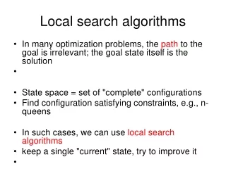
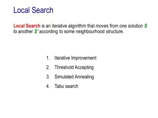
Local Search. Local Search is an iterative algorithm that moves from one solution S to another S′ according to some neighbourhood structure. 1. Iterative Improvement 2. Threshold Accepting 3. Simulated Annealing 4. Tabu search. General Local Search Procedure. Initialisation .

E N D
Local Search Local Searchis an iterative algorithm that moves from one solution S to another S′ according to some neighbourhood structure. 1. Iterative Improvement 2. Threshold Accepting 3. Simulated Annealing 4. Tabu search
General Local Search Procedure • Initialisation. • Neighbour Generation. • Acceptance Test. • Termination Test. Choose an initial schedule Sto be the current solution and compute the value of the objective function F(S). Select a neighbour S’ of the current solution S and compute F(S’). Test whether to accept the move from S to S’. If the move is accepted, then S’ replaces S as the current solution; otherwise S is retained as the current solution. Test whether the algorithm should terminate. If it terminates, output the best solution generated; otherwise, return to the neighbour generation step.
General Local Search Procedure Transpose neighbourhood: (1,2,3,4,5,6,7) (1,3,2,4,5,6,7) Swap neighbourhood: (1,2,3,4,5,6,7) (1,6,3,4,5, 2,7) Insert neighbourhood: (1,2,3,4,5,6,7) (1,3,4,5,6, 2,7) • Initialisation. • Neighbour Generation. • Acceptance Test. • Termination Test. Random permutation (J1, J2, … , Jn) for single-machine problem or flow-shop, more complicated structures for other models. Neighbours may be generated randomly, systematically, or by some combination of the two approaches. Specific for each type of local search algorithm Limited computation time or the number of iterations
General Local Search Procedure In Step 3, the acceptance rule is usually based on values F(S) and F(S′) of the objective function for schedules S and S′. In some algorithms only moves to “better” schedules are accepted (schedule S′ is better than Sif F(S′)< F(S)) In others it may be allowed to move to “worse” schedules. Sometimes “wait and see” approach is adopted. The algorithm terminates in Step 4 if the computation time exceeds the limit or after completing the established number of iterations or if no further improvements are possible.
1. Iterative Improvement As described As described As described The algorithm can be applied repeatedly starting each time with a different randomly generated initial solution. • Initialisation. • Neighbour Generation. • Acceptance Test. • Termination Test. Choose S’ only if F(S’)<F(S) (strict improvement in the objective function value)
2. Threshold Accepting As described As described As described Allows to continue the local search even if a local optimum has been obtained • Initialisation. • Neighbour Generation. • Acceptance Test. • Termination Test. Choose S’ if F(S’)-F(S)<a, where a >0 is a threshold value. Usually a is relatively large at the beginning, becomes smaller later on.
3. Simulated Annealing As described As described As described • Initialisation. • Neighbour Generation. • Acceptance Test. • Termination Test. Probabilistic acceptance test
3. Simulated Annealing Probabilistic Acceptance Test: Determine D= F(S’) - F(S). • If D0, then a move to schedule S’ is always accepted. • If D>0, then a move to schedule S’ is accepted with probability e-D/T, where T is a parameter called the temperature, which changes during the course of the algorithm. Usually T is large in the beginning and then it decreases until it is close to 0 at the final stages. Different “cooling schemes” can be applied. Often Tk= ak, where Tkis the temperature at iteration k and 0<a<1.
“Cycling” of SA and TA • It is possible to get back to the solutions already visited • A simple way to avoid such problems is to store all visited solutions in a list called tabu list. • A new solution can be accepted if it is not contained in the list.
4. Tabu Search (TS) As described As described As described • Initialisation. • Neighbour Generation. • Acceptance Test. • Termination Test. • A “worse” schedule S’ may be accepted • Deterministic acceptance test based on tabu list
4. Tabu Search (TS) Tabu List • Tabu list stores attributes of the previous few moves. • It has a fixed number of entries (usually between 5 and 9). • It is updated each time S’ is accepted: • the reverse transformation is entered at the top of tabu list to avoid returning to the same solution (to avoid returning to a local optimum); • all other entries are pushed down one position; • the bottom entry is deleted.
4. Tabu Search (TS) Deterministic Acceptance Test: Determine D= F(S’) - F(S). - If D<0 and S’ is “non-tabu”, then a move to S’ is always accepted - If D<0 and S’ is “tabu”, then a move to S’ may be accepted for a “promising” schedule S’ (if F(S’) is less than the objective function value for any other solution obtained before) - If D0 and S’ is “tabu”, then a move to S’ is always rejected. - If D 0 and S’ is “non-tabu”, then a “wait and see” approach is adopted: S’ remains as a candidate while the search continues for a neighbour which can be accepted immediately. If no such neighbour is found, a move to the best candidate S’ is made.
Conclusions • Local search algorithms are very generic. • They have been applied successfully to many industrial problems. • Performance of local search algorithms depends on construction of neighborhood. • A method that exploits special structure is usually faster (if one exists).
Intensification vs Diversification • Intensification mechanisms aim to carefully examine a specific area of the search space in order to find a higher-quality solution. Intensification is often achieved by adopting a greedy approach (the search is directed to the best possible neighbour). • Diversification mechanisms aim to explore the search space widely in order to avoid the search stagnation. • An important issue in the design of a local search method is to achieve a good balance between intensification and diversification.
Local Search Process TA TS SA B&B, Iterative Improvement