Local search algorithms
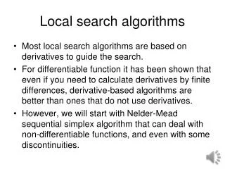
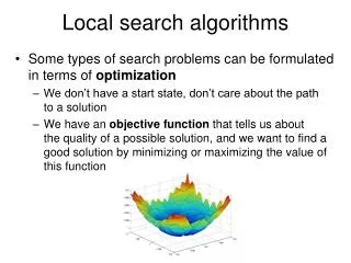
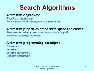
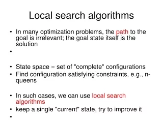
Local search algorithms. In many optimization problems, the state space is the space of all possible complete solutions We have an objective function that tells us how “good” a given state is, and we want to find the solution (goal) by minimizing or maximizing the value of this function.

Local search algorithms
E N D
Presentation Transcript
Local search algorithms • In many optimization problems, the state space is the space of all possible complete solutions • We have an objective function that tells us how “good” a given state is, and we want to find the solution (goal) by minimizing or maximizing the value of this function
Example: n-queens problem • Put n queens on an n × n board with no two queens on the same row, column, or diagonal • State space: all possible n-queen configurations • What’s the objective function? • Number of pairwise conflicts
Example: Traveling salesman problem • Find the shortest tour connecting a given set of cities • State space: all possible tours • Objective function: length of tour
Local search algorithms • In many optimization problems, the state space is the space of all possible complete solutions • We have an objective function that tells us how “good” a given state is, and we want to find the solution (goal) by minimizing or maximizing the value of this function • The start state may not be specified • The path to the goal doesn’t matter • In such cases, we can use local search algorithms thatkeep a single “current” state and gradually try to improve it
Example: n-queens problem • Put n queens on an n × n board with no two queens on the same row, column, or diagonal State space: all possible n-queen configurations • Objective function: number of pairwise conflicts • What’s a possible local improvement strategy? • Move one queen within its column to reduce conflicts
Example: n-queens problem • Put n queens on an n × n board with no two queens on the same row, column, or diagonal State space: all possible n-queen configurations • Objective function: number of pairwise conflicts • What’s a possible local improvement strategy? • Move one queen within its column to reduce conflicts h = 17
Example: Traveling Salesman Problem • Find the shortest tour connecting n cities • State space: all possible tours • Objective function: length of tour • What’s a possible local improvement strategy? • Start with any complete tour, perform pairwise exchanges
Hill-climbing search • Initialize current to starting state • Loop: • Let next= highest-valued successor of current • If value(next) < value(current) return current • Else let current = next • Variants: choose first better successor, randomly choose among better successors • “Like climbing mount Everest in thick fog with amnesia”
Hill-climbing search • Is it complete/optimal? • No – can get stuck in local optima • Example: local optimum for the 8-queens problem h = 1
The state space “landscape” • How to escape local maxima? • Random restart hill-climbing • What about “shoulders”? • What about “plateaux”?
Simulated annealing search • Idea: escape local maxima by allowing some "bad" moves but gradually decrease their frequency • Probability of taking downhill move decreases with number of iterations, steepness of downhill move • Controlled by annealing schedule • Inspired by tempering of glass, metal
Simulated annealing search • Initializecurrentto starting state • For i = 1 to • If T(i) = 0 return current • Let next = random successor of current • Let = value(next) – value(current) • If > 0 then let current = next • Else let current = next with probability exp(/T(i))
Effect of temperature exp(/T)
Simulated annealing search • One can prove: If temperature decreases slowly enough, then simulated annealing search will find a global optimum with probability approaching one • However: • This usually takes impractically long • The more downhill steps you need to escape a local optimum, the less likely you are to make all of them in a row • More modern techniques: general family of Markov Chain Monte Carlo (MCMC) algorithms for exploring complicated state spaces
Local beam search • Start with k randomly generated states • At each iteration, all the successors of all k states are generated • If any one is a goal state, stop; else select the k best successors from the complete list and repeat • Is this the same as running k greedy searches in parallel? Greedy search Beam search