Download
1 / 14
140 likes | 266 Vues
This study explores entropy production in highly transparent colliding systems, focusing on the LHC's energy transition from 158 GeV to 14000 GeV. It discusses the role of thermodynamic principles in particle interactions under anisotropic conditions, emphasizing the need for a continuum framework that accommodates anisotropy to understand the thermodynamic state of the matter produced in high-energy collisions. The article presents theoretical formulations and equations governing the entropy-to-particle number ratio, internal energy, and heat currents relevant in these collisional scenarios.

E N D
ENTROPY PRODUCTION IN HIGHLY TRANSPARENT COLLIDING SYSTEMS • B. Lukács • CRIP RMKI
The LHC, Geneva, is almost 2 orders of magnitude increase in beam energy. • However, how much is it in enmtropy? (In continuum physics S is more important than E!) • So how much S/N is expected at 7000+7000 GeV E/N?
Note that: • S/N was 50±5 at 158 GeV E/A fixed target (≈9+9 GeV E/N). (Rafelski, Letessier and Tounsi, several times from yields) • Ebeam is not the internal energy. • Ordered motion does not produce S!
Also, carefully, because • S is a par excellence thermodynamical quantity; • But the internal state of the matter is very anisotropic. • The cross-sections are very forward-peaked at such energies, so after a few collisions the particles move still almost unperturbed (so S/N cannot be big).
So we need thermodynamics with an extra anisotropy degree of freedom so that S=0 at undisturbed ambidirectional flow of any velocities • + • A relativistically exact anisotropic continuum dynamics. • Let us do it!
THE FORMALISM [1] B. Lukács & K. Martinás: Dynamically Redundant Particle Components in Mixtures. Acta Phys. Slov. 36, 81 (1986) [2] H-W. Barz, B. Kämpfer, B. Lukács, K. Martinás & G. Wolf: Deconfinement Transition in Anisotropic Matter. Phys. Lett. 194B, 15 (1987) [3] H-W. Barz, B. Kämpfer, B. Lukács & G. Wolf: Anisotropic Nuclear Matter with Momentum-Dependent Interactions. Europhys. Lett. 8, 239 (1989) [4] B. Kämpfer, B. Lukács, K. Martinás & H-W. Barz: Fluid Dynamics in Anisotropic Media. KFKI-1990-47 [5] H-W. Barz, B. Kämpfer, B. Lukács & G. Wolf: Obobshennaya gidrodinamika vzaimopronikayushchih potokov yadernoi materii. Yad. Phys. 51, 366 (1990) [6] B. Kämpfer, B. Lukács, G. Wolf & H-W. Barz: Description of the Stopping Process within Anisotropic Thermodynamics. Phys. Lett. 240B, 237 (1990) Almost archaeology. However…
You cannot be sure in too much; but • Tir;r = 0 • nr;r = 0 • sr;r≥ 0 • And that will be enough!
Tik = αuiuk + β(uitk+tiuk) + γtitk + (diuk+uidk) + (bitk+tibk) + cik drur = drtr = brur = brtr = cirur = cirtr = 0 Vector di is heat current; local equilibrium approach neglects it. If so, we may neglect bi as well. We may assume that cik (a 2*2 tensor) is “as isotropic as possible”. Tik = euiuk + β(uitk+tiuk) + k{gik+uiuk-titk/t2} where we wrote α→e due to the usual definition Tikuiuk ≡ e
β is 0 in a mirror-symmetric state, see [5]. Then si = sui + zti Let us see z later. Vector anisotropy is ti . It is in beam direction. Its length is t. The extent of anisotropy is t, so let the anisotropy extensive be Q = Vnt = Vq= Vnt and the proper thermodynamical potential density s s = s(e,n,q) By change of variable š ≡ š(e,n,t) = s(e,n,q=nt)
š,tDt + (š-nš,n-eš,e-kš,e)ur;r + tr(z,r-š,eβ,r) + tr;r(z-š,eβ) – š,eβtrusur;s - š,e(γ-k/t2)trtsur;s ≥ 0 D ≡ us∂s identically; and it holds identically only if the coefficients satisfy k = p(e,n,t) + ωTš,t +δur;r p = T(š -nš,n-eš,e) z = β/T ω ≥ 0 δ ≥ 0 1/T ≡ š,e
So Dt = λ + ν(T,r+Tur;sus)tr + θtrtsur;s + ωur;r š,tλ ≥ 0 ν = β/T2š,t θ = (k/t2-γ)/š,t As well we can take the approximation ω=δ=0. Then λ is the only new quantity governing “thermalisation”.
Then we have got the full system of evolution eqs. as: Dn + nur;r = 0 De + (e+p+q)ur;r = 0 Du + {D(p+q) + (p+q),x}/(e+p+q) = 0 Dq + (q+q/v)ur;r - λ = 0 where q = nt.
Equation of state: for a nuclear matter with ideal gas + compression + pion gas with fully relativistic ambidirectional flow: p = nT + (π2/30)T4 + (K/9)n0x2(varctgv – 1 + x(2/y – y)) e = mny + (3/2)nT + (π2/10)T4 + (K/18)n(x-1)2 + (K/9)n(y-1)(x/y2((y+1)(x/y – 1) + (1 – x2/y)/2) q = mxn0ln(v+y) + (K/9)n0((x/2)ln(v+y) – x2arctgv + vx2((3x/2y) -1/y2 – xv2/y3)) y ≡ (1+v2)1/2 x ≡ n/n0 where –v/T is the intensive conjugate to Q ≡ Vq.
We are just integrating and calculating yields (that is another matter going back to 1991 in thermodynamics) with A. Steer.