Marc Riedel
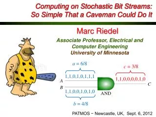
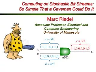
Computing on Stochastic Bit Streams: So Simple That a Caveman Could Do It. Marc Riedel. a = 6/8. c = 3/8. Associate Professor, Electrical and Computer Engineering University of Minnesota. 1,1,0,1,0,1,1,1. b = 4/8. 1,1,0,0,0,0,1,0. 1,1,0,0,1,0,1,0. Non-Polynomial Functions.

Marc Riedel
E N D
Presentation Transcript
Computing on Stochastic Bit Streams:So Simple That a Caveman Could Do It Marc Riedel a = 6/8 c = 3/8 Associate Professor, Electrical and Computer Engineering University of Minnesota 1,1,0,1,0,1,1,1 b = 4/8 1,1,0,0,0,0,1,0 1,1,0,0,1,0,1,0
Non-Polynomial Functions Find a Bernstein polynomial with coefficients in the unit interval that approximates the non-polynomial g(t). Find real values to minimize Solved by quadratic programming subject to
Example: Gamma Correction Function Coefficients of Degree-6 Bernstein polynomial approximation: b0,6 = 0.0955, b1,6 = 0.7207, b2,6 = 0.3476, b3,6 = 0.9988, b4,6 = 0.7017, b5,6 = 0.9695, b6,6 = 0.9939
Fault Tolerance • Stochastic Encoding • A bit flip does not substantially change the probability: 1010111001 → 1010011001 • Binary Radix Encoding • A bit flip in the most significant bit causes a huge change in the value: (1010)2 → (0010)2 0.6 0.5 10 2
Fault Tolerance Implementing arithmetic function y=x1x2s+x3(1−s) for x1=4/8, x2=6/8, x3=7/8 and s=2/8. 10% noise injection. StochasticImplementation Small error! DeterministicImplementation Large error!
Deterministic v.s. Stochastic Implementation of Gamma correction function with 10% noise injection. Deterministic implementation:37% pixels with errors > 25% 1% 2% 10% Conventional Implementation Stochastic Implementation: no pixels with errors > 25%! Stochastic Implementation
Hardware Cost Comparison • Compare conventional implementation to stochastic implementation of polynomial functions. • Mapped onto FPGA (counting the number of LUTs) • Conventional implementation: 10-bit binary radix • Stochastic implementation: bit stream of length 210
Comparison of Fault Tolerance for Mathematical Functions Sixth-order Maclaurin polynomial approx., 10 bits: sin(x), cos(x), tan(x), arcsin(x), arctan(x), sinh(x), cosh(x), tanh(x), arcsinh(x), exp(x), ln(x+1)
Sequential Constructs What about complex functions such as tanh, exp, and abs?
Sensing Applications Median Filter-Based Image Noise Reduction
Sensing Applications Frame Difference-Based Image Segmentation
Sensing Applications Image Contrast Enhancing
Sensing Applications Kernel Density Estimation-Based Image Segmentation
General Approach for Generating Stochastic Bit Streams R probability to be one 0, 1, 1, 0, 1, … If R < C, output a one; If R ≥ C, output a zero. Comparator C
Types of Random Sources • Psuedorandom Number Generator Linear Feedback Shift Register (expensive) • Physical Random Source Thermal Noises (cheap)
Challenge withPhysical Random Sources cheap Voltage Regulators expensive expensive C2 C1 Suppose many differentprobabilities are needed:{0.2, 0.78, 0.2549, 0.43, 0.671, 0.012, 0.82, …}. It is costly to generate them directly.(many expensive constant values required.)
Opportunity with Physical Random Sources cheap 1,1,0,0,0, … 0,1,0,1,0, … 0,0,1,0,1, … expensive • Independent • Same probability
Solution When we need many different probabilities: {0.2, 0.78, 0.2549, 0.43, 0.671, 0.012, 0.82, …} • Generate a few probabilities directly from physical random sources. • Synthesize combinational logic to generate other probabilities. Probability: Probability of a signal being logical one
Basic Problem Set S of Input Probabilities{p1 , p2} Set S of Input Probabilities{p1 , p2} Other Probabilities Needed q1 q2 q3 p1 p1 q4 p1 p1 … p1 p1 RandomSources Independent p2 p2 p2 p2 LogicCircuit … p2 p2 • Synthesize Logic Circuit? (|S| small) • Choose Set S?
Example 0.4 0.6 … 0.4 0.2 0.5 … 0.3 0.5 P(x = 1) = 0.4 P(x = 1) = 0.4 0,0,1,0,1,0,1,0,1,0 0,1,0,1,0,0,1,1,0,0 P(z = 1) = 0.3 P(z = 1) = 0.2 P(z = 1) = 0.6 P(x = 1) = 0.4 0,1,0,0,0,1,0,0,0,1 0,0,0,1,0,0,1,0,0,0 LogicCircuit 1,0,1,1,0,1,0,0,0,0 0,1,0,0,1,0,1,1,1,1 1,0,0,1,1,0,0,1,1,0 1,0,1,1,0,0,1,0,0,1 P(y = 1) = 0.5 P(y = 1) = 0.5 P(z = 1) = P(x = 0) P(z = 1) = P(x = 0) P(y = 0) P(z = 1) = P(x = 1) P(y = 1)
Generating Decimal Probabilities Decimal Probabilities Choose Set S = {p1, p2, p3} q1 q2 … q3 p1 q4 Independent … p1 p2 … p2 p3 LogicCircuit p3 • Found Set S for • |S| = 2 • |S| = 1 Large Cost! |S| Small!
Generating Decimal Probabilities Theorem: With S = {0.4, 0.5}, we can synthesize arbitrarydecimal output probabilities. • Constructive proof. • Derived a synthesis algorithm. “The synthesis of combinational logic to generate probabilities” W. Qian, M. Riedel, K. Barzagan, and D. Lilja International Conference on Computer-Aided Design, 2009 Best Paper Award Nomination
Algorithm Example: Synthesize q = 0.757 from S= {0.4, 0.5} (Black dots are inverters) 1 − ×0.4 1 − ×0.5 1 − ×0.5 0.6075 0.43 0.3925 0.785 0.215 0.757 0.243 For a probability value with n digits, need at most 3n AND. 1 − ×0.5 1 − ×0.5 1 − ×0.5 ×0.4 0.14 0.86 0.4 0.6 0.3 0.7 0.35
combinationallogic Generating Decimal Probabilities Question: Does there exist a set S of size one which can generate arbitrary decimal probabilities? p p Independent q p p Yes! (p irrational, p ≈ 0.1295)
Implementation • Focus on generating decimal probability formS = {0.4, 0.5}. • Goal: Reduce circuit depth.
Precision versus Bit Length • Stochastic encoding • Uniform and not compact: To represent 2n different values, need 2n bits • Binary radix encoding • Positional and compact: To represent 2n different values, need n bits For applications that can tolerate small error, we don’t need a large n.
Error due to Stochastic Variance • x = P(X = 1) = 2/5 → 0,1,0,1,1 (x= 3/5) • Increasing the length of bit streams reduces the error. • Effect of errors is uniform and small. • Target application: low precision, e.g., hardware for sensing appication operating in harsh environments.
Comparison of Encoding (Positional, Weighted) (Uniform) (Uniform,Long Stream) (Positional) (Compact, Efficient) (Not compact, Long Stream) Binary Radix Encoding Stochastic Encoding Spectrum of Encoding
Future Directions Spectrum of Encoding ? Binary Radix Encoding(Compact, Positional) Stochastic Encoding (Not compact, Uniform) Possible encodings in the middle with theadvantages of both?