Modeling Curved Surfaces
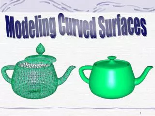
Modeling Curved Surfaces. Curved Surfaces. The use of curved surfaces allows for a higher level of modeling, especially for the construction of highly realistic models. There are several approaches to modeling curved surfaces:. (1) Similar to polyhedral models ,

Modeling Curved Surfaces
E N D
Presentation Transcript
Curved Surfaces The use of curved surfaces allows for a higher level of modeling, especially for the construction of highly realistic models. There are several approaches to modeling curved surfaces: (1) Similar to polyhedral models, we model an object by using small curved surface patches(instead of polygons) placed next to each other. (2) Another approach is solid modeling, that constructs a model using elementary solid objects (such as: polyhedra, spheres, cones etc.) as building blocks.
Curved Surfaces There are two ways to construct a model: Additive Modeling This is the process of building the model by assembling many simpler objects. Subtractive Modeling This is the process of removing pieces from a given object to create a new object. For example, creating a (cylindrical) hole in a sphere or a cube. We can represent curved surfaces using mesh of curves. So we learn to create curves first then move to curved surfaces. Curved Surface Patch
Curve Representation • There are three ways to represent a curve • Explicit: y = f(x) y = mx + b y = x2 (–) Must be a single valued function (–) Vertical lines, say x = d? • Implicit: f(x,y) = 0 x2 + y2 - r2 = 0 (+) y can be multiple valued function of x (–) Vertical lines? • Parametric: (x, y) = (x(t), y(t)) (x, y) = (cost, sint) (+) Easy to specify, modify and control (–) Extra hidden variable t, the parameter
Explicit Representation • Curve in 2D: y = f(x) • Curve in 3D: y = f(x), z = g(x) • Surface in 3D: z = f(x,y) • Problems: • How about a vertical line x = c as y = f(x)? • Circle y = (r2 – x2)1/2 two or zero values for x • • Rarely used in computer graphics
Implicit Representation • Curve in 2D: f(x,y) = 0 • Line: ax + by + c = 0 • Circle: x2 + y2 – r2 = 0 • Surface in 3d: f(x,y,z) = 0 • Plane: ax + by + cz + d = 0 • Sphere: x2 + y2 + z2 – r2 = 0 • f(x,y,z) can describe 3D object: • Inside: f(x,y,z) < 0 • Surface: f(x,y,z) = 0 • Outside: f(x,y,z) > 0
Parametric Form for Curves • Curves: single parameter u (e.g. time) • x = x(t), y = y(t), z = z(t) • Circle: • x = cos(t), y = sin(t), z = 0 • Tangent described by derivative • Magnitude is “velocity”
Parametric Form for Surfaces • Use parameters u and v • x = x(u,v), y = y(u,v), z = z(u,v) • Describes surface as both u and v vary • Partial derivatives describe tangent plane at each point p(u,v) = [x(u,v) y(u,v) z(u,v)]T
Advantages of Parametric Form • Parameters often have natural meaning • Easy to define and calculate • Tangent and normal • Curves segments (for example, 0 u 1) • Surface patches (for example, 0 u,v 1)
Lagrange Polynomial • Given n+1 points (x0, y0), (x1, y1) …….. (xn, yn) • To construct a curve that passes through these points we can use Lagrange polynomial defined as follows:. Problems: • y=f(x), no multiple values • Higher order functions tend to oscillate • No local control (change any (xi, yi) changes the whole curve) • Computationally expensive due to high degree.
Piecewise Linear Polynomial • To overcome the problems with Lagrange polynomial • Divide given points into overlap sequences of 4 points • construct 3rd degree polynomial that passes through these points, p0, p1 , p2 , p3 then p3, p4 , p5 , p6 etc. • Then glue the curves so that they appear sufficiently smooth at joint points. • Questions: • Why 3rd Degree curves used? • How to measure smoothness at joint point?
Why Cubic Curves? A curve is approximated by a piecewise polynomial curve. Cubic polynomials are most often used because: (1) Lower-degree polynomials offer too little flexibility in controlling the shape of the curve. (2) Higher-degree polynomials can introduce unwanted wiggles and also require more computation. (3) No lower-degree representation allows a curve segment to be defined by two given endpoints with given derivative at each endpoints. (4) No lower-degree curves are nonplanar in 3D.
Measure of Smoothness G0 GeometricContinuity C0 ParametricContinuity If two curve segments join together. C0 G1 GeometricContinuity If the directions (but not necessarily the magnitudes) of the two segments’ tangent vectors are equal at a join point. C1 ParametricContinuity If the directions and magnitudes of the two segments’ tangent vectors are equal at a join point. C1 C2ParametricContinuity If the direction and magnitude of Q2(t) (curvature or acceleration) are equal at the join point. CnParametricContinuity C2 If the direction and magnitude of Qn(t) through the nth derivative are equal at the join point.
Measure of Smoothness C2 Joint Point C1 S C0 TV3=2*TV1 TV2=TV1 Q3 Q2 Q1 • By increasing parametric continuity we can increase smoothness of the curve. • Q1& Q2 are C1 and G1 continuous • Q1& Q3 are G1 continuous only as Tangent vectors have different magnitude. • Observe the effect of increasing in magnitude of TV P0
Desirable Properties of a Curve • Simple control • lines need only two points • curves will need more (but not significantly more) • Intuitive control • Physically meaningful quantities like position, tangent, curvature etc. • Global Vs. Local Control • Portion of curve effected by a control point. • General Parameterization • Handle multi-valued x-y mapping
Desirable Properties of a Curve cont’d • Interpolation Vs Approximation • Axis Independent • Equation might change but the shape remain same under a coordinate transform • (translation, rotation, scaling) of a curve = (translation, rotation, scaling) of its control points. • Degree of Smoothness. • May need more or less • May need varying degrees of smoothness in a single curve.
Interpolation Vs. Approximation Given n + 1 points P0(x0, y0), P1(x1, y1), …, Pn(xn, yn) we wish to find a curve that, in some sense, fits the shape outlined by these points. Based on requirements we are faced with two problems: Interpolation If we require the curve to pass through all the points. Approximation If we require only that the curve be near these points.
Parametric Representation of Lines P1 P2 Blending Function B Parameter T Basis Matrix M Geometry G Co-eff C • Interpolation of two points • In Parametric form:
Parametric Cubic Curves é ù a a a x y z ê ú b b b [ ] ( ) ê ú x y z \ = 3 2 Q t t t t 1 ê ú c c c x y z ê ú T d d d ê ú ë û x y z C ( ) \ = × Q t T C
Parametric Cubic Curves é ù é ù m m m m G 11 12 13 14 1 ê ú ê ú [ ] m m m m G ê ú ê ú 21 22 23 24 2 = 3 2 Q ( t ) t t t 1 ê ú ê ú m m m m G 31 32 33 34 3 ê ú ê ú m m m m G ë û ë û 41 42 43 44 4 geometry basis matr ix vector • Now co-efficient matrix C can be expressed as a multiple of basis(weight) matrix M and geometry matrix G. [ ] ( ) ( ) ( ) ( ) = = × = × × Q t x t y t z t T C T M G • Each element of geometry vector G has 3 component for x, y and z. • Components of G can be expressed as Gx, Gy and Gz.
Parametric Cubic Curves ( ) = + + + 3 2 x t t m t m tm m g 11 21 31 41 1 x ( ) + + + + 3 2 t m t m tm m g 12 22 32 42 2 x ( ) + + + + 3 2 t m t m tm m g 13 23 33 43 3 x ( ) + + + + 3 2 t m t m tm m g 14 24 34 44 4 x a blending function • Multiplying out only the x-component we get é ù é ù m m m m g 11 12 13 14 1 x ê ú ê ú [ ] m m m m g ê ú ê ú 21 22 23 24 2 x = × × = 3 2 x ( t ) T M G t t t 1 ê ú ê ú x m m m m g 31 32 33 34 3 x ê ú ê ú m m m m g ë û ë û 41 42 43 44 4 x ( ) • The curve is a weighted sum of the elements of geometry matrix • The weights are each cubic polynomials of t calledblending function
Derivative of Q(t) • Derivative of Q(t) is the parametric tangent vector of the curve.
Curve Design : Determining C A curve segment Q(t) is defined by constraints on: (1) endpoints (2) tangent vectors and (3) continuity between segments Each cubic polynomial of Q(t) has 4 coefficients, so 4 constraints will be needed, allowing us to formulate 4 equations in the 4 unknowns, then solving for the unknowns.
Hermit Curves R4 R1 P4 P1 A cubic Hermite curve segment interpolating the endpoints P1 and P4 is determined by constraints on the endpoints P1 and P4 and tangent vectors at the endpoints R1 and R4
Hermit Curves The Hermite Geometry Vector: The constraints on x(0) and x(1):
Hermit Curves Hence the tangent-vector constraints: The 4 constraints can be written as:
Hermit Curves f(t) P1 P4 1 R1 t 1 R4 The Hermite Blending Functions
Bézier Curves P2 P4 P1 P3 Indirectly specifies the endpoint tangent vectors by specifying two intermediate points that are not on the curve.
Bézier Curves The Bézier Geometry Vector:
Bézier Curves The 4 polynomials in BB = T . MB are called the Bernstein polynomials.
Bézier Curves f(t) 1 t 1 The Bernstein Polynomials A Bézier curve is bounded by the convex hull of its control points.
What's a Spline? • Smooth curve defined by some control points • Moving the control points changes the curve
Other Curves • Natural Cubic Spline • C0, C1 and C2 continuous cubic polynomial • Smoother than previous curves which don’t have C2 continuity. • Interpolates all of the control points • B-Splines • C0, C1 and C2 continuous cubic polynomial • Don’t interpolate the control points • Varieties: • Uniform Vs Nonuniform • Rational Vs Non-rational • Catmull-Rom splines • And many more….
Catmull-Rom Splines ( ) = × × Q t T M G CR Bs i - é ù é ù P 2 2 1 1 - i 2 ê ú ê ú - - - P 3 3 2 1 ê ú ê ú - i 1 = T ê ú ê ú - ( P P ) 2 0 0 1 0 - - i 1 i 3 ê ú ê ú - ( P P ) 2 1 0 0 0 ë û ë û - i i 2 Hermite Basis - - é ù é ù P 1 3 3 1 Q(0) - i 3 ê ú ê ú Q(1) - - P 2 5 4 1 1 ê ú ê ú - i 2 = × × T ê ú ê ú - P 1 0 1 0 2 - i 1 ê ú ê ú P 0 2 0 0 ë û ë û i • Interpolation splines i.e. Passes through all control points. • Tangent at any control point is parallel to the line joining the control points adjacent to that point.
Curve Rendering • Brute-Force method • Forward differencing • Recursive sub-division Brute-Force method t = 0; for (i=0; i <= 100; i++) { x(t) = axt3+ bxt2+ cxt+ dx y(t) = ayt3+ byt2+ cyt+ dy x(t) = azt3+ bzt2+ czt+ dz Plot3d( x(t), y(t), z(t) ); t += 0.01;}
Curve Rendering Forward differencing method
Curve Rendering Forward differencing method = 1 / n; f =d; f = a3+ b3+ c; f 2= 6a3+ 2b2; f 3= 6a3; Plot(f.x, f.y, f.z ); for (i=0; i <= n; i++) { f += f ; f += f 2; f 2+= f 3; Plot(f.x, f.y, f.z ); }
Curve Rendering P2 d3 P4 P1 d2 P3 Straight if d2 < and d3 < Recursive sub-division Void DrawCurveRecSub(curve, ) { if (Straight(curve, ) DrawLine(curve); else { SubdivideCurve(curve, leftCurve, rightCurve); DrawCurveRecSub(leftCurve, ); DrawCurveRecSub(RightCurve, ); } }
Planer Surfaces • Using bi-linear interpolation
Parametric Bicubic Surfaces • Generalization of parametric cubic curves • The elements of geometry matrix are curves themselves instead of constants.
Hermite Surfaces • Harmite Surfaces are completely defined by a 4X4 geometry Matrix GH • The surface is a stacking of (s) Curves • Each (s) curve is a Harmite Curve • With end points and end tangents as function of (t)
Hermite Surface P(1,1) P(0,1) t P(1,0) P(0,0) s
