Comprehensive Statistical Analysis with R Software
Learn how to use R software for statistical analysis. Follow simple steps for data entry, functions, object manipulation, and file handling. Access resources from the R project website. Start your R journey now!

Comprehensive Statistical Analysis with R Software
E N D
Presentation Transcript
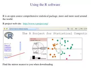
Using the R software R is an open source comprehensive statistical package, more and more used around the world. R project web site: http://www.r-project.org/ Find the mirror nearest to you when downloading
Install with PDF Manual included !! Check this box! (All boxes can be checked if you have enough memory space.)
R comes with no typical menu selection graphical user interface (GUI) All must be entered at command level (or by writing scripts). Entering data Functions:c, matrix, cbind, data.frame, read.table Help on functions available i R GUI from Help R functions (text) …
Entering data from keyboard Example: We want to enter the vector x = (1, 2) and the matrix To enter something (whatever) we use the assignment operator “<-” Assigning a vector: The function c() combines individual values (comma-spaced) to a vector
Printing the value on screen: Either enter the variable or use the function print() Note that the output begins with [1]. This is the row number, and in this case x is interpreted as a row vector Listing defined objects (vectors, matrices, data frames): Use the function ls() with no arguments
What if we just use ls ? The source code of the function ls() is printed on screen
Removing objects: Use the function rm() (Enter x again: )
Assigning a matrix: Alternative 1: Use the function matrix() a<-matrix(values,nrow=m,ncol=n) values is a list of values enclosed in c(), i.e. a row vector or an already defined vector. m is the number of rows and n is the number of columns of the matrix. The number of values must be dividable by both m and n. The values are entered column-wise. The identifiers nrow= and ncol= can be omitted Note the double indexing, first number for row and second number for column
Identifiers skipped If row and column numbers are “erroneously” specified: Note! There is a result, though, but the fourth value is omitted.
Alternative 2: Concatenating (already existing) columns Use the function cbind() …with already existing columns (vectors): Note! The columns will now be indexed by the original column (vector) names
Collecting vectors and matrices with the same number of rows in a data frame Use the function data.frame(object 1, object 2, … , object k) Matrices need to be protected , otherwise each column of a matrix will be identified as a single object in the data frame. Protection is made with the function I()
Objcets within a data frame can be called upon using the syntax dataframe$object
Names of objects within a data frame can be called, set or changed by handling the object names()
Reading from an external data file Assume we have our data stored on the file demo.dat in directory D:\undv\732A26 x a.1 a.2 1 2 1 2 1 -1 Set correct working directory in R: Note! Path must be specified with slashes (/) which is Unix-language and not backslashes (\) which is DOS-language. To see which is the current working directory:
To read from the file, use the function read.table(filename,header=logical_value,sep=separator) filename is the name of the file enclosed with double quotes ( ” ” ). It can be specified with the whole path if it is not in the current working directory logical_value is set to TRUE if the columns in the file have headers, otherwise it should be set to FALSE (it is set automatically if omitted, but the result may be “unexpected”) separator is set to the separator sign for the columns in the file, (default is ” ” for blank-separated columns)
Note!read.table treats every column of the file as an individual column, i.e. it cannot be used to read a matrix directly into the workspace The columns of a stored matrix must be recombined to create the matrix
Writing to an external file The function write.table(dataframe,filename,append=logical_value,sep=logical_value, quote=logical_value,row.names=logical_value,col.names=logical_value) can be used for different formats of the output dataframe is the name of the data frame to be written on file filename is the name of the file to write to logical_value is either TRUE or FALSE If append=FALSE (default) a file will be created and any existing file with that name will be destroyed. If append=TRUE the data frame will be added (vertical concatenation) to an existing file.
Examples: Exploring demo1.dat with Notepad (“Anteckningar” in Swedish) Row numbers!
Tab-separated, but the first header do not correspond vertically with the first column. The first column of the file is the row number.
(append=FALSE is default and can therefore be omitted for new file creation) Row numbers have now been removed and headers correspond vertically with the columns.
Note! Multiple lines can be used for a command input. A carriage return before the command is completed opens a new line with the prompt “+” Column names (headers) have been removed.
Calculation The ordinary arithmetic operators “+”, “–”, “*” and “/” work element-wise
Matrix operators/functions: transpose b=t(a) b = aT inverse b=solve(a)b = a-1 (when needed) QR-factorization qr=qr(a) Additional arguments possible qr.Q(qr) Q qr.R(qr) R x=qr.solve(A,b) Solves A·x = b
Alternatively: “reg” becomes an object as output from qr This object has a number of members (coef, res, fitted)
A more comprehensive regression analysis is done with the function lm() (linear model) Use help(”lm”) to learn more about this function
Putting it together in a script Gather command rows in a text file..Give it extension “.r” Call the script file with command source a<-matrix(c(2,1,1,-1),2,2) b<-c(1,2) x=qr.solve(a,b) print(x) Store in d:\undv\732A26\macro.r “#” precedes a comment
When exiting R Workspace can be saved for future sessions: save.image(”core.RData”) saves the workspace into file core.RData where core is replaced by a suitable filename base. To restore a saved workspace: load(”core.RData”) To exit from R type q()
More programming Regular sequences: Note! ”<-” can be reversed and most often ”<-” can be replaced by ”=”
Repeating patterns Note! Identifier needs to be specified (times or each)
Conditions must be within parentheses. Normally: Put “else” directly after “}”
Equality condition must be given with operator ”==” Multiple statements following a for, if, else or while must be separated by semicolon (;) runif(1) gives a random U(0,1) number General usage: runif(n,a,b) n is the number of values, default: a=0, b=1
A more complex example:Simulating regression data Script: x1=c(2,3,5,6,9,10,10,12,13,15) # First x-variable x2=c(1,0,0,1,0,1,1,0,1,1) # Second x-variable y<-as.numeric(1:10) # Dimensioning y for (i in (1:10)) { # Computing y using beta1=1.1 and beta2=-4.7 # Random error is N(0,2) y[i]=12+1.1*x1[i]-4.7*x2[i]+rnorm(1,0,2) } Plot(x1,y) # generates a scatter plot y vs. x1 # Estimating the coefficients: x=cbind(rep(1,each=10),x1,x2) b=qr.solve(x,y) print(b) Store in file regress.r
Suppose we would like to get empirically derived confidence limits for 1 , i.e. not using the normal distribution. beta1<-as.numeric(1:500) # Dimensioning array of b1-values x1=c(2,3,5,6,9,10,10,12,13,15) # First x-variable x2=c(1,0,0,1,0,1,1,0,1,1) # Second x-variable y<-as.numeric(1:10) # Dimensioning y for (trial in 1:500) { for (i in (1:10)) { # Computing y using beta1=1.1 and beta2=-4.7 # Random error is N(0,2) y[i]=12+1.1*x1[i]-4.7*x2[i]+rnorm(1,0,2) } # Estimating the coefficients: x=cbind(rep(1,each=10),x1,x2) b=qr.solve(x,y) # Storing b1 in array beta1[trial]=b[2] } Store in file regress2.r
Bootstrapping the estimated 90th percentile of a sample Assume we wish to assess the 90th percentile of a sample from a Poisson distribution. This means that we wish to assess the properties opf the sample percentile as an estimator of the population percentile in terms of bias 95% confidence Simulate a sample of 40 observations from a Po(7)-distribution, show an initial histogram of the sample values. Draw 500 pseudo-samples with replacement from the original sample In each pseudo-sample, compute the sample percentile Collect the pseudo-sample percentiles, translate them by subtracting the original sample percentile and estimate bias and 95% percentile confidence limits