Download
1 / 28
280 likes | 390 Vues
Employing GIS to investigate karst regions: A quantitative assessment. Eric W. Peterson Brianne Jacoby Illinois State University Toby Dogwiler Winona State University. Importance. Landforms provide clues to how a cave developed

E N D
Employing GIS to investigate karst regions: A quantitative assessment Eric W. Peterson Brianne Jacoby Illinois State University Toby Dogwiler Winona State University
Importance • Landforms provide clues to how a cave developed • Provide insight to paleoenvironments through understanding past base levels and upstream events • Glaciations • Tectonics
Sediment Dating • Sediment accumulates in caves once it is abandoned by flow • Date 26Al and 10Be to learn the timing of deposition • Timing can correlate with surface events that affected a region’s climate and geomorphology history
Level Studies • Mammoth Cave1 • Cumberland Plateau2 • Both studies used sediment dating and found four levels present • Both mentioned the possibility of a fifth level • Similar Geology • Similar Timing • Incision during the Pliocene-Pleistocene Glaciations 1Granger et al, 2001 2Anthony and Granger, 2004.
Level Development • Passages created at static flow and correlate to passages at similar elevations are collectively considered a level • Form from active dissolution during static base level elevation • Abandoned once incision increases and the base level lowers • Location where horizontal flow transitioned to rapid incision (Piezometric limit)
Objectives • Use GIS to determine time associated with cave level development • Determine if cave levels are correlated to Stream Power Index (SPI)
General Geology and Hydrogeology • 106 km2 of deeply incised valleys • Fluviokarst • 3 bedrock formations • Borden Formation (oldest) • Shale • Newman Formation • Limestone • Pennington Formation (capping unit) • Sandstone • Tygarts Creek is the local base level (flows north to the Ohio River)
Levels of CCSRP The ends of the boxes represent the 25th and 75th percentiles with the solid line at the median and the dashed line at the mean; the error bars depict the 10th and 90th percentiles and the points represent outliers. Mean increases with age level. Numerical values can be found in Table 2.
Spatial Distribution 4 Levels (Option 1) 5 Levels (Option 2)
Methods • Materials: • GIS • Cave Opening Data • 10-meter DEM • 3D Analysis tool used to calculate area and volume • Used denudation rates from the literature to calculate time • Computed SPI coverage results for all levels and stratigraphy in both DEMs
How the 3D Tool Works • Blue Line Represents Level Elevation • Red Stippled Area Represents the area and volume being calculated
Area and Volume • Total Level Volume = (volume beneath top of level) – (volume beneath base of level) • Total Thickness Lost = (Level Volume/Level Area) • Time = (Thickness Lost)/(Denudation Rate)
Denudation Rates • The act of lowering the landscape through erosion • A rate of 30 m/Ma is accepted for the Appalachians
Comparison 1Granger et al, 2001 2Peterson, et al (in review) 3Anthony and Granger, 2004, and White, 2007 4Ma B.P. stands for millions of years before present.
What is SPI? (Stream Power Index) • Digital terrain analysis • Uses a digital elevation model (DEM) • Determines erosive power of flowing water based on slope and flow accumulation • No measurement of discharge required • Relies on quality of digital data and little field work
Slope • For each cell, the slope tool calculates the maximum rate of change between it and its neighbors • Identifies the steepest downhill slope √(dz/dx)2 + (dz/dy)2) = slope
Flow Accumulation and SPI • SPI = Slope * Flow Accumulation based on elevation Sum of cells that flow into a single cell
Conclusions • Greatest volume, area, and material lost in levels at highest elevations and oldest in age. These also took the longest to develop • 4 rates between 12 and 40 m/Ma • Average rate is 24 m/Ma • Higher erosion potential at lower elevations • Higher SPI threshold coverage in limestone than clastic rocks