Ordinal and Multinomial Models
Ordinal and Multinomial Models. William Simpson Research Computing Services. http://intranet.hbs.edu/dept/research/statistics/. Types of Models. Models are generalizations of the logit and probit models Ordinal logit and probit deal with ordered data (more than 2 categories)


Ordinal and Multinomial Models
E N D
Presentation Transcript
Ordinal and Multinomial Models William Simpson Research Computing Services http://intranet.hbs.edu/dept/research/statistics/
Types of Models • Models are generalizations of the logit and probit models • Ordinal logit and probit deal with ordered data (more than 2 categories) • Multinomial logit deals with unordered data with more than 2 categories • (Multinomial probit is not commonly used due to computational difficulties)
Outline of Talk • Review of Binary Models • Ordinal Models • Multinomial Logit
Binary Data – View 1 (CDF) • View 1 – we compute a number that is a linear combination of our predictors, call it y=+ x. We then convert y into a probability p by using a cumulative distribution function (CDF). Our final outcome is 1 with probability p.
Binary Data – View 2 (Latent or Unobserved Variable) • View 2 – we compute a number that is a linear combination of our predictors and then add an error term, call it y*= + x+ u We then get an outcome of 1 if y* >= 0, outcome 0if y* < 0. In this case, the probabilistic element is the error term u, and y* is an unobserved variable.
Binary Data – Unobserved Variable View PDF of Y*
What Happens When Standard Deviation of u Changes y*= + x+ v std(v) > std(u)
Comparing CDF and Latent Variable Views • The two views are equivalent. Each one can be converted into the other, where the cumulative probability function (CDF) in view 1 matches the CDF of the distribution of u in view 2.
Ordinal Outcomes • 3 or more categorical outcomes, which can be treated as ordered • Bond ratings (AAA, AA, … B, C, …) • Likert scales (e.g. responses on a 1-7 scale, from strongly disagree to strongly agree) • Often analyzed as continuous
SAS and Stata Code Stata oprobit outcome x or ologit outcome x SAS proc logistic; class outcome; model outcome = x / link=probit; or model outcome = x ; run;
Sample Output (Stata oprobit) --------------------------------------------------------- y | Coef. Std. Err. z P>|z| --------------------------------------------------------- x | 1.074575 .1209108 8.89 0.000 -------------+------------------------------------------- _cut1 | -2.076242 .1548201 (Ancillary parameters) _cut2 | -.9736895 .0807119 _cut3 | -.4528313 .073509 _cut4 | 1.106628 .0781733 _cut5 | 2.079342 .0932966 _cut6 | 3.176076 .167065 ----------------------------------------------------------
Interpretation of Stata Output x | 1.074575 .1209108 -------------+----------------------- _cut1 | -2.076242 .1548201 _cut2 | -.9736895 .0807119 • Outcome will be in the second ordered category or higher (not the first), if 1.07*x+u > -2.08. • Outcome will be in the third ordered category or higher (not the first or second), if 1.07*x+u > -.97. • Outcome will be in the second ordered category exactly, if -.97 > 1.07*x+u > -2.08.
Sample Output (SAS PROC LOGISTIC with LINK=PROBIT) Parameter DF Estimate Std Error Intercept 71 -3.17580.1666 Intercept 61 -2.07930.0933 Intercept 51 -1.10660.0781 Intercept 410.45280.0734 Intercept 310.97370.0807 Intercept 212.07620.1555 x 11.07460.1208
Interpretation of SAS Output • Outcome will be in the second ordered category or higher (not the first), if 1.07*x + 2.08 + u > 0. • Outcome will be in the third ordered category or higher, if 1.07*x + .97 + u > 0. • Outcome will be in the second ordered category if 1.07*x + 2.08 + u > 0 and 1.07*x + .97 + u < 0. Intercept 310.97370.0807 Intercept 212.07620.1555 x 11.07460.1208
Interpreting Coefficients • Multiple cutpoints with no intercept term, or multiple intercept terms • Probabilities modeled are probabilities for all outcomes >=k, compared with all outcomes < k. • Interpret the coefficients the same as in the corresponding binary model.
Assumptions of Ordinal Models • Relationship between probabilities and + x follows the assumed form (normal for probit, logistic for logit). • Parallel regressions – Coefficient is the same for every hurdle – aka equal slopes, (proportional odds for logistic models) • If not, use generalized ordered logit
Sample Likert Scalewith Extra Points 2.3 4.2 1 2 3 4 5 6 7 ----------------------------------------------------------- SD D SoD N SoA A SA MoD VSA SD=Strongly Disagree, SoD = Somewhat Disagree D=Disagree, N=Neutral, A=Agree SA=Strongly Agree, SoA=Somewhat Agree MoD=Moderately Disagree VSA = Very Slightly Agree
Sample Likert Scalewith Uneven Points 1 2 3 4 5 6 7 ----------------------------------------------------------- SD D MoD SoD N VSA SA (1) (2) (2.3) (3) (4) (4.2) (7) SD=Strongly Disagree, SoD = Somewhat Disagree MoD=Moderately Disagree D=Disagree, N=Neutral VSA = Very Slightly Agree SA=Strongly Agree
Multinomial Logit • A generalization of logistic regression • More than two outcomes • Outcomes are not ordered • We are interested in the relative probabilities of outcomes
Examples • Choice of transportation – bus, taxi, private car • Choice of product brand • Occupational choice (considered as unordered) – craft, blue collar, professional, white collar
Sample Results ----------------------------------------------------- outcome | Coef. Std. Err. z P>|z| -------------+--------------------------------------- Taxi | distance | -.0757664 .1305456 -0.58 0.562 income | .319901 .0830162 3.85 0.000 _cons | -6.22562 1.734012 -3.59 0.000 -------------+--------------------------------------- Car | distance | .4482523 .1129979 3.97 0.000 income | .0447404 .0581754 0.77 0.442 _cons | -2.587764 1.214103 -2.13 0.033 ----------------------------------------------------- (Outcome outcome==Bus is the comparison group)
Sample Results (2) ----------------------------------------------------- outcome | Coef. Std. Err. z P>|z| -------------+--------------------------------------- Bus | distance | .0757664 .1305456 0.58 0.562 income | -.319901 .0830162 -3.85 0.000 _cons | 6.22562 1.734012 3.59 0.000 -------------+--------------------------------------- Car | distance | .5240187 .1245058 4.21 0.000 income | -.2751607 .080734 -3.41 0.001 _cons | 3.637855 1.705811 2.13 0.033 ----------------------------------------------------- (Outcome outcome==Taxi is the comparison group)
Taxi Bus Bus Taxi Bus Car Taxi Car .0757664 -.0757664 .4482523 .5240187 Coefficients on Distance Bus Taxi + Taxi Car = Bus Car -.0757664 + .5240187 = .4482523 Bus Car=Taxi Car – Taxi Bus
Independence from Irrelevant Alternatives (IIA) • Relative odds of two categories shouldn’t change when a new category is added • E.g., if choices are car, bus, and Yellow Cab, the relative proportions shouldn’t change if a new choice is added, e.g. Black & White Cab • Not realistic in this case. Assumption should be examined carefully.
Other Models for Nominal Outcomes • Conditional Logit • Attributes of choices can be used as predictors • Nested Logit • Treats a set of choices as a hierarchy • IIA assumption can be relaxed
References • Long, J. S. (1997). Regression Models for Categorical and Limited Dependent Variables. Thousand Oaks, CA: Sage. • Hosmer, D. W. and S. Lemeshow. (2000). Applied Logistic Regression (Second ed.). New York: Wiley. • Allison, P. D. (1999). Logistic Regression Using the SAS System: Theory and Application. Cary, NC: SAS Institute. • Long, J. S. & Freese, J. (2001). Regression Models for Categorical Dependent Variables using Stata. College Station, TX: Stata Press.
Appendix Programming Examples By James Zeitler
Ordered Logit (SAS) proclogistic data = work.ordinals descending; model y = x; run; The LOGISTIC Procedure Model Information Data Set WORK.ORDINALS .............................................. Model cumulative logit Optimization Technique Fisher's scoring Response Profile Ordered Total Value y Frequency 1 7 6 ............................. 7 1 6 Probabilities modeled are cumulated over the lower Ordered Values. Analysis of Maximum Likelihood Estimates Standard Wald Parameter DF Estimate Error Chi-Square Pr > ChiSq Intercept 7 1 -6.1912 0.4312 206.1863 <.0001 Intercept 6 1 -3.6194 0.1804 402.7389 <.0001 Intercept 5 1 -1.8611 0.1414 173.2883 <.0001 Intercept 4 1 0.7326 0.1275 33.0150 <.0001 Intercept 3 1 1.7093 0.1520 126.4030 <.0001 Intercept 2 1 4.3014 0.4189 105.4418 <.0001 x 1 1.8479 0.2176 72.1016 <.0001
Ordered Probit (SAS) proclogistic data = work.ordinals descending; model y = X / LINK = PROBIT; run; The LOGISTIC Procedure Model Information Data Set WORK.ORDINALS ............................................... Model cumulative probit Response Profile Ordered Total Value y Frequency 1 7 6 ............................ 7 1 6 Probabilities modeled are cumulated over the lower Ordered Values. Analysis of Maximum Likelihood Estimates Standard Wald Parameter DF Estimate Error Chi-Square Pr > ChiSq Intercept 7 1 -3.1758 0.1666 363.5568 <.0001 Intercept 6 1 -2.0793 0.0933 496.5331 <.0001 Intercept 5 1 -1.1066 0.0781 200.8158 <.0001 Intercept 4 1 0.4528 0.0734 38.0347 <.0001 Intercept 3 1 0.9737 0.0807 145.4615 <.0001 Intercept 2 1 2.0762 0.1555 178.1792 <.0001 x 1 1.0746 0.1208 79.1034 <.0001
Multinomial Logit (SAS) /* Use Link = GLOGIT in PROC LOGIT */ /* to estimate a multinomial logit */ /* Refer to the response profile to */ /* determine the reference category */ proclogistic data = transport; class Mode; model Mode = Distance Income /link = glogit; run; The LOGISTIC Procedure Model Information Data Set WORK.TRANSPORT Response Variable Mode Number of Response Levels 3 Model generalized logit Response Profile Ordered Total Value Mode Frequency 1 Bus 27 2 Car 42 3 Taxi 31 Logits modeled use Mode='Taxi' as the reference category. Analysis of Maximum Likelihood Estimates Standard Wald Parameter Mode DF Estimate Error Chi-Square Pr > ChiSq Intercept Bus 1 6.2253 1.7340 12.8897 0.0003 Intercept Car 1 3.6375 1.7057 4.5475 0.0330 Distance Bus 1 0.0757 0.1305 0.3367 0.5617 Distance Car 1 0.5240 0.1245 17.7135 <.0001 Income Bus 1 -0.3199 0.0830 14.8488 0.0001 Income Car 1 -0.2751 0.0807 11.6155 0.0007