
SlideServe
Menu
Préférences
© SlideServe · v2026

Multinomial Distributions

cleopatra avatar
12 diapositives · 520 Views · Mar 08, 2014

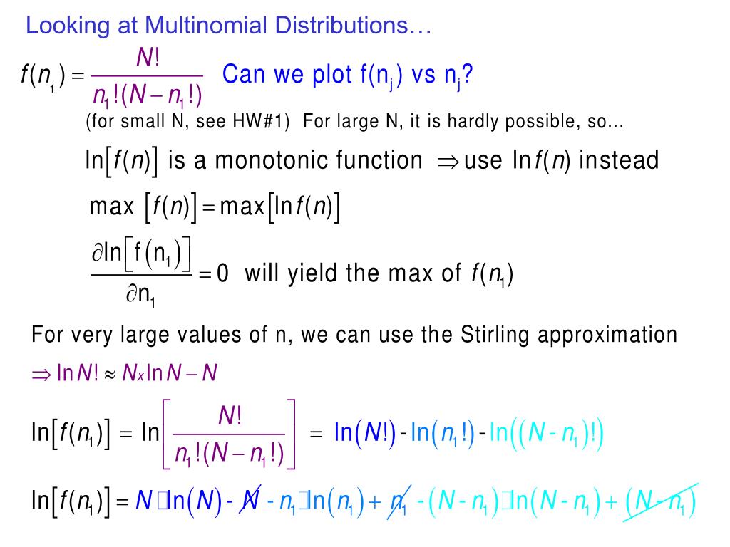
Multinomial Distributions. Looking at Multinomial Distributions…. Maximum of a distribution. Shape of a Distribution. Plots Distributions. So far, we look at a function with a single variable n 1. Constraints in the distributions.
Multinomial Distributions - slide 1
01 / 12Multinomial Distributions
1 / 17

Télécharger la présentation

Multinomial Distributions
Une image / un lien ci-dessous est fourni (tel quel) pour télécharger la présentation

Politique de téléchargement : le contenu du site vous est fourni TEL QUEL pour votre information et votre usage personnel ; il ne peut être vendu, concédé sous licence ni partagé sur d’autres sites sans l’accord de son auteur.Le contenu vous est fourni TEL QUEL, pour votre information et votre usage personnel uniquement. Téléchargez la présentation en cliquant sur ce lien. Lors du téléchargement, si vous ne parvenez pas à télécharger une présentation, l’éditeur a peut-être supprimé le fichier de son serveur.Pendant le téléchargement, si vous ne parvenez pas à obtenir une présentation, le fichier a peut-être été supprimé par l’éditeur.

F I N

Plus de contenu associé

Transcription de la présentation
  1. Multinomial Distributions Looking at Multinomial Distributions…

  2. Maximum of a distribution

  3. Shape of a Distribution

  4. Plots Distributions

  5. So far, we look at a function with a single variable n1. Constraints in the distributions How to maximize a function of multiple variables, when the variables are not independent? (n1n2 n3 etc) i.e maximize the Multinomial distribution with Snj = const.

  6. undetermined multiplier Lagrange Undetermined Multipliers Lagrange multipliers

  7. Lagrange multipliersII

  8. First Law E1 E2 Some “old” Thermo, to remember our roots… Extensive properties depend on the system size (V, S, mass, etc) Intensive properties do not depend on syst. Size (T, p, etc) Isolated systems evolve SPONTANEOUSLY toward simple “terminal states” (equilibrium). • 1st Law: • Internal energy is extensive E1+ E2 =E • E is conserved ( changes are the result of doing something to the system (dE = dQ+dw) X = extensive mechan. properties. Change in X involves work Adiabatic walls control exchange of heat Equilibrium is macroscopically characterized by (E,X)  a small number of control variables

  9. Second Law Equilibrium is reached (kept) by constraints. What terminal state will be reached if a constraint is removed or changed? Entropy: Extensive property, S(E,X) 2nd Law: If state B can be adiabatically reached from state A, then SBSA • A process which can be exactly retraced by infinitesimal changes in its control variables reversible • arbitrarily slowly moving from one equilibrium state to another  trajectory within the manifold of equilibrium states • Natural processes do not proceed through the manifold of equilibrium states cannot be retraced irreversible

  10. If AB is adiabatic SBSA and if it is also reversible, then BA is also adiabatic  SASB Second law II  SA = SB for adiabatically reversible processes If AB is irreversible, BA cannot be reached adiabaticallythen SB>SA DS 0 for adiabatic process

  11. S(E,X) Entropy properties which also holds for reversible non-adiabatic processes, because S, E and X are functions of state

  12. intensive extensive Temperature