Download
1 / 69
690 likes | 913 Vues
Teaching Data Analysis as an Investigative Process with Census at School. Rebecca Nichols and Martha Aliaga American Statistical Association. US Census at School Program. Free international classroom project that engages students in grades 4-12 in statistical problem solving

E N D
Teaching Data Analysis as an Investigative Process with Census at School Rebecca Nichols and Martha Aliaga American Statistical Association
US Census at School Program Free international classroom project that engages students in grades 4-12 in statistical problem solving Students complete an online survey, analyze their class census data, and compare their class results with random samples of participating students in the United States and other countries. The project began in the United Kingdom in 2000 and includes Australia, Canada, New Zealand, South Africa, Ireland, Japan, and now the United States. Teach statistical concepts in the Common Core Standards, measurement, graphing, data analysis, and statistical problem solving in context of students’ own data and data from their peers in the participating countries www.amstat.org/censusatschool
Statistical Problem Solving Guidelines for Assessment and Instruction in Statistics Education (GAISE) Report: A Pre-K–12 Curriculum Framework 1. Formulate Questions • Clarify the problem at hand • Formulate one (or more) questions that can be answered with data 2. Collect Data • Design a plan to collect appropriate data • Employ the plan to collect the data 3. Analyze Data • Select appropriate graphical and numerical methods • Use the methods to analyze the data 4. Interpret results • Interpret the analysis (in context) • Relate the interpretation to the original question Source: www.amstat.org/education/gaise
Common Core State Standards for Mathematics Source: corestandards.org
Measurement & Data – Grades 4 & 5 Grade 4 (4.MD) Measurement and Data Strand – Common Core State Standards • Solve problems involving measurement and conversion of measurements from a larger unit to a smaller unit. • Represent and interpret data. Grade 5 (5.MD) Measurement and Data • Convert like measurement units within a given measurement system. • Represent and interpret data. The U.S. Census at School questionnaire includes measurement questions (measuring height, arms pan, and foot length in centimeters, finger length in millimeters, etc.) and opportunities to represent and interpret real student data. Source: corestandards.org
Statistics & Probability – Grade 6 (6.SP) Develop understanding of statistical variability 1. Recognize a statistical question as one that anticipates variability in the data related to the question and accounts for it in the answers. For example, “How old am I?” is not a statistical question, but “How old are the students in my school?” is a statistical question because one anticipates variability in students’ ages. 2. Understand that a set of data collected to answer a statistical question has a distribution which can be described by its center, spread, and overall shape. 3. Recognize that a measure of center for a numerical data set summarizes all of its values with a single number, while a measure of variation describes how its values vary with a single number. Source: corestandards.org
Statistics & Probability – Grade 6 (6.SP) Develop understanding of statistical variability 1. Recognize a statistical question as one that anticipates variability in the data related to the question and accounts for it in the answers. For example, “How old am I?” is not a statistical question, but “How old are the students in my school?” is a statistical question because one anticipates variability in students’ ages. 2. Understand that a set of data collected to answer a statistical question has a distribution which can be described by its center, spread, and overall shape. 3. Recognize that a measure of center for a numerical data set summarizes all of its values with a single number, while a measure of variation describes how its values vary with a single number. Source: corestandards.org
Statistics & Probability – Grade 6 (6.SP) Summarize and describe distributions 4. Display numerical data in plots on a number line, including dot plots, histograms, and box plots. 5. Summarize numerical data sets in relation to their context, such as by: • Reporting the number of observations. • Describing the nature of the attribute under investigation, including how it was measured and its units of measurement. • Giving quantitative measures of center (median and/or mean) and variability (interquartile range and/or mean absolute deviation), as well as describing any overall pattern and any striking deviations from the overall pattern with reference to the context in which the data were gathered. • Relating the choice of measures of center and variability to the shape of the data distribution and the context in which the data were gathered. Source: corestandards.org
Statistics & Probability – Grade 7 (7.SP) Use random sampling to draw inferences about a population 1. Understand that statistics can be used to gain information about a population by examining a sample of the population; generalizations about a population from a sample are valid only if the sample is representative of that population. Understand that random sampling tends to produce representative samples and support valid inferences. 2. Use data from a random sample to draw inferences about a population with an unknown characteristic of interest. Generate multiple samples (or simulated samples) of the same size to gauge the variation in estimates or predictions. For example, estimate the mean word length in a book by randomly sampling words from the book; predict the winner of a school election based on randomly sampled survey data. Gauge how far off the estimate or prediction might be. Source: corestandards.org
Statistics & Probability – Grade 7 (7.SP) Draw informal comparative inferences about two populations 3. Informally assess the degree of visual overlap of two numerical data distributions with similar variabilities, measuring the difference between the centers by expressing it as a multiple of a measure of variability. For example, the mean height of players on the basketball team is 10 cm greater than the mean height of players on the soccer team, about twice the variability (mean absolute deviation) on either team; on a dot plot, the separation between the two distributions of heights is noticeable. 4. Use measures of center and measures of variability for numerical data from random samples to draw informal comparative inferences about two populations. For example, decide whether the words in a chapter of a seventh-grade science book are generally longer than the words in a chapter of a fourth-grade science book. Note: Grade 7 also includes probability standards Source: corestandards.org
Statistics & Probability – Grade 8 (8.SP) Investigate patterns of association in bivariate data 1. Construct and interpret scatter plots for bivariate measurement data to investigate patterns of association between two quantities. Describe patterns such as clustering, outliers, positive or negative association, linear association, and nonlinear association. 2. Know that straight lines are widely used to model relationships between two quantitative variables. For scatter plots that suggest a linear association, informally fit a straight line, and informally assess the model fit by judging the closeness of the data points to the line. 3. Use the equation of a linear model to solve problems in the context of bivariate measurement data, interpreting the slope and intercept. For example, in a linear model for a biology experiment, interpret a slope of 1.5 cm/hr as meaning that an additional hour of sunlight each day is associated with an additional 1.5 cm in mature plant height. Source: corestandards.org
Statistics & Probability – Grade 8 (8.SP) Investigate patterns of association in bivariate data 4. Understand that patterns of association can also be seen in bivariate categorical data by displaying frequencies and relative frequencies in a two-way table. Construct and interpret a two-way table summarizing data on two categorical variables collected from the same subjects. Use relative frequencies calculated for rows or columns to describe possible association between the two variables. For example, collect data from students in your class on whether or not they have a curfew on school nights and whether or not they have assigned chores at home. Is there evidence that those who have a curfew also tend to have chores? Source: corestandards.org
Statistics & Probability – High SchoolInterpreting Categorical & Quantitative Data (S-ID) Summarize, represent, and interpret data on a single count or measurement variable 1. Represent data with plots on the real number line (dot plots, histograms, and box plots). 2. Use statistics appropriate to the shape of the data distribution to compare center (median, mean) and spread (interquartile range, standard deviation) of two or more different data sets. 3. Interpret differences in shape, center, and spread in the context of the data sets, accounting for possible effects of extreme data points (outliers). 4. Use the mean and standard deviation of a data set to fit it to a normal distribution and to estimate population percentages. Recognize that there are data sets for which such a procedure is not appropriate. Use calculators, spreadsheets, and tables to estimate areas under the normal curve. Source: corestandards.org
Statistics & Probability – High SchoolInterpreting Categorical & Quantitative Data (S-ID) Summarize, represent, and interpret data on two categorical and quantitative variables 5. Summarize categorical data for two categories in two-way frequency tables. Interpret relative frequencies in the context of the data (including joint, marginal, and conditional relative frequencies). Recognize possible associations and trends in the data. 6. Represent data on two quantitative variables on a scatter plot, and describe how the variables are related. a. Fit a function to the data; use functions fitted to data to solve problems in the context of the data. Use given functions or choose a function suggested by the context. Emphasize linear, quadratic, and exponential models. b. Informally assess the fit of a function by plotting and analyzing residuals. c. Fit a linear function for a scatter plot that suggests a linear association. Source: corestandards.org
Statistics & Probability – High SchoolInterpreting Categorical & Quantitative Data (S-ID) Interpret linear models 7. Interpret the slope (rate of change) and the intercept (constant term) of a linear model in the context of the data. 8. Compute (using technology) and interpret the correlation coefficient of a linear fit. 9. Distinguish between correlation and causation. Source: corestandards.org
Statistics & Probability – High SchoolMaking Inferences & Justifying Conclusions (S-IC) Understand and evaluate random processes underlying statistical experiments 1. Understand statistics as a process for making inferences about population parameters based on a random sample from that population. 2. Decide if a specified model is consistent with results from a given data-generating process, e.g., using simulation. For example, a model says a spinning coin falls heads up with probability 0.5. Would a result of 5 tails in a row cause you to question the model? Source: corestandards.org
Statistics & Probability – High SchoolMaking Inferences & Justifying Conclusions (S-IC) Make inferences and justify conclusions from sample surveys, experiments, and observational studies 3. Recognize the purposes of and differences among sample surveys, experiments, and observational studies; explain how randomization relates to each. 4. Use data from a sample survey to estimate a population mean or proportion; develop a margin of error through the use of simulation models for random sampling. 5. Use data from a randomized experiment to compare two treatments; use simulations to decide if differences between parameters are significant. 6. Evaluate reports based on data. Source: corestandards.org
US Census at School Program www.amstat.org/censusatschool
US Census at School Program Free international classroom project that engages students in grades 4-12 in statistical problem solving Students complete an online survey, analyze their class census data, and compare their class results with random samples of participating students in the United States and other countries. The project began in the United Kingdom in 2000 and includes Australia, Canada, New Zealand, South Africa, Ireland, Japan, and now the United States. Teach statistical concepts in the Common Core Standards, measurement, graphing, data analysis, and statistical problem solving in context of students’ own data and data from their peers in the participating countries www.amstat.org/censusatschool
US Census at School Program Students complete a brief online survey (classroom census) 13 international questions plus additional U.S. questions 15-20 minute computer session Analyze your class results Use teacher password to gain immediate access to class data Formulate questions of interest that can be answered with Census at School data, collect/select appropriate data, analyze the data with appropriate graphs and numerical summaries, internet the results, and make appropriate conclusions in context relating to the original questions Compare your class with samples from the U.S. and other countries Download a random sample of Census at School data from U.S. students Download a random sample from participating international students International lesson plans are available, along with instructional webinars and other free resources www.amstat.org/censusatschool
US Census at School Program www.amstat.org/censusatschool
US Census at School – Student Section www.amstat.org/censusatschool
US Census at School – Student Section www.amstat.org/censusatschool
US Census at School – Teacher Section www.amstat.org/censusatschool
US Census at School – Resources www.amstat.org/censusatschool
US Census at School Random Sampler www.amstat.org/censusatschool
International Random Sampler www.amstat.org/censusatschool
Statistical Investigations - Census at School Formulate statistical questions of interest that can be answered with the Census at School data. Collect/select appropriate Census at School data and write down the variable names and type for this investigation. Analyze the data. Include appropriate graphs and numerical summaries for the corresponding variables. Interpret the results and make appropriate conclusions in context. Be sure to justify your results using your graphs and numerical summaries and relate your interpretation to the original question. For a demonstration of this process and software resources (some free) to analyze the data, watch the Census at School webinars posted under Resources at www.amstat.org/censusatschool.
Formulating a Statistical Question Common Core Standards – Grade 6 (6.SP) 1. Recognize a statistical question as one that anticipates variability in the data related to the question and accounts for it in the answers. For example, “How old am I?” is not a statistical question, but “How old are the students in my school?” is a statistical question because one anticipates variability in students’ ages. A well-written statistical question anticipates answers that will vary and includes: • Population of interest • Measurement of interest Example from Common Core: How old are the students in my school? • Population of interest: Students in my school • Measurement: Age (measured in years) • Student ages will vary
Formulate Statistical Questions Example Statistical Questions with Census at School • How much time per week do students participating in U.S. Census at School spend on the computer? • Population of interest: Students (grades 4-12) participating in U.S. Census at School • Measurement: Time on the computer each week (measured in hours) • Time (hours per week) will vary by student • What is the favorite sport /activity of students in Australia participating in Census at School? • Population of interest: Students in Australia participating in U.S. Census at School • Measurement: Favorite sport (baseball, basketball, bowling, etc.) • Favorite sport/activity will vary by student • Is there a difference between the reaction times of boys and girls (participating in U.S. Census at School)? • Populations/groups of interest: Boys and girls participating in U.S. Census at School • Measurement: Reaction time (measured in seconds) • Reaction times will vary by student
Formulate Statistical Questions Example Statistical Questions with Census at School • Is there a relationship between height and arm span for students participating in Census at School? • Population of interest: Students participating in U.S. Census at School • Measurements: Height (measured in cm) and arm span (measured in cm) • Measured heights and arm spans will vary by student • Does the preferred superpower of U.S. Census at School students differ by gender? • Populations/groups of interest: Boys and girls participating in U.S. C@S • Measurement: Preferred superpower (categories: fly, freeze time, invisibility, super strength, telepathy) • Preferred superpower will vary by student • Does travel time to school vary by country for the students participating in Census at School? • Populations/groups of interest: Students participating in C@S in the various countries • Measurement: Travel time to school (measured in minutes) • Measured heights and arm spans will vary by student
Collect/Select Census at School Data • Download your class data • Download random samples of other students in the U.S. participating in Census at School with the online U.S. Census at School Random Sampler • Download random samples of students in other countries participating in Census at School with the online International Census at School Random Sampler • Select the variables of interest needed to investigate the statistical question and write down the variable names and type for this investigation • Because the Census at School data comes from real students and is entered online by these students, there will be some mistakes and inappropriate data values in the data sets. Before analyzing your data and making conclusions, make sure to take time to observe and clean your data. Create a graph for each variable of interest to look for inappropriate or unusual values that do not make sense in context of the variable and original survey question.
Analyze & Interpret C@S Data For the statistical questions: • Create appropriate graphs • Create numerical summaries • Apply the concepts in the Common Core State Standards (or state standards) with real student data • Interpret the results and make appropriate conclusions in context. Be sure to justify your results using your graphs and numerical summaries and relate your interpretation to the original question. • We will review appropriate graphs, numerical summaries, and interpretations in context of Census at School data.
Review: Variables • Variable – Any characteristic whose value may change from one individual/object to another. • Quantitative (Numerical, Measurement) Variable: • Census at School Examples: • Age: 13 years • Height: 138 cm (measured in cm since it is an international program) • Travel time to school: 15 minutes • Categorical (Qualitative) Variable: • Census at School Examples: • Country: Australia/Canada/New Zealand/South Africa/United Kingdom/USA • Gender: Male/Female • Handed: Right handed/Left handed/Ambidextrous • Why does the type of variable matter?
Graphical Displays by Type of Variable • One Quantitative Variable • Dot plot • Stem & leaf plot • Histogram • Box & whisker plot (box plot) • One Categorical Variable: • Bar graph (preferred) • Circle graph/Pie chart
Bar Charts vs. Histograms • Horizontal axis is categorical. • Shape, center, and spread have no meaning in a bar chart. • Space usually separates each bar. • Horizontal axis is quantitative. • Histograms are described by shape, center, and spread. • Bars are usually adjacent.
Numerical Summaries by Type of Variable • Quantitative data: • Mean (measure of center appropriate for symmetric data) • Median (measure of center not as influenced by skewness & outliers as the mean) • Standard deviation (measure of spread appropriate when using mean as a measure of center, similar to mean absolute deviation) • Interquartile range (measure of spread appropriate when using median as a measure of center, less influenced by skewness and outliers) • Range (measure of spread) • Others • Categorical data: • Counts/frequencies • Percentages • Modal category Use the graphs and numerical summaries appropriate for your grade level(s).
Central Cluster Bell Left Cluster Skewed Right Right Cluster Skewed Left Two Clusters Bimodal Flat Uniform 1 2 5 3 5 4 5 5 5 6 5 5 70% 80% 90% 100% - 3 - 2 - 1 0 1 2 3 4 5 6 7 4 0 3 0 y c n e u 2 0 q e r F 1 0 0 -6 -3 3 -9 9 6 0 0 0 Interpreting Graphs for One Quantitative Variable (Histogram, Dot Plot, Stem & Leaf Plot, Box & Whisker Plot) Shape Center Spread
Interpreting Graphs (One Quantitative Variable) • Shape (bell-shaped, skewed, flat/uniform, etc.) • Center (mean, median) • Spread/Variability (standard deviation, mean absolute deviation, interquartile range, range) • Possible outliers
Interpreting Graphs (One Quantitative Variable) Shape Center Spread/Variability Possible outliers These values (0, 1 and 20 cm) fall outside the overall pattern and are not plausible heights (the world’s shortest person is 50 cm).
Interpreting Graphs (One Quantitative Variable) Shape symmetric, bell-shaped Center Spread/Variability Possible outliers
Interpreting Graphs (One Quantitative Variable) Shape Center mean ≈ median since shape approx.symmetric Spread/Variability Possible outliers
Interpreting Graphs (One Quantitative Variable) Shape Center Spread/Variability (standard deviation, interquartile range, range) Range – distance between the maximum and minimum values The outliers were not included in this case since they are not possible height values .
Interpreting Graphs (One Quantitative Variable) Shape Center Spread/Variability (standard deviation, interquartile range, range) Interquartile range = Q3 – Q1, range of the middle 50% of values
Interpreting Graphs (One Quantitative Variable) Shape Center Spread/Variability (standard deviation, interquartile range, range) Standard Deviation – an average distance of observations from the mean (similar to mean absolute deviation)
Interpreting Graphs for One Quantitative Variable Census at School Example Variable: Height Bell-shaped, symmetric Shape Center Mean height = 157.6 cm Median height = 158 cm Standard deviation of heights = 13.5 cm (an average distance from the mean height is 13.5 cm) Interquartile range of heights = Q3 – Q1 = 167 – 149 = 18 cm (range of the middle 50% of heights is 18 cm) Range of heights = Max – Min= 200 – 116 = 84 cm Spread
Interpreting Graphs for One Quantitative Variable Census at School Example: Importance of Saving Energy Rating Scale 0 to 1000 Left-skewed Shape Center Median rating = 699 Mean rating = 678.2 Standard deviation of ratings = 282.1 (an average distance from the mean rating is 282.1) Interquartile range of ratings = Q3-Q1 = 999–500= 499 (range of the middle 50% of ratings is 499) Range of ratings =Max-Min= 1000–0= 1000 Spread
Interpreting Graphs for One Quantitative Variable Census at School Example Variable: Travel Time to School Right-skewed Shape Center Median travel time = 15 minutes Mean travel time = 18.1 minutes Standard deviation = 14.3 minutes (an average distance from the mean travel time is 14.3 minutes) Interquartile Range = Q3-Q1= 25–7= 18 minutes (range of the middle 50% of travel times is 18 minutes) Range =Max-Min= 70–1= 69 minutes Spread
Graphical Displays for Two Variables • Two Quantitative Variables • Scatter plot • Two Categorical Variables • Tables • Two variable bar charts • One Quantitative and One Categorical Variable • Side by side dot plots • Side by side box & whisker plots (works well for multiple groups – strength of box plots) • Back to back stem & leaf plots (Compare distribution of quantitative variable for two groups)
Two Quantitative Variables Scatter Plot Examples: Is there a relationship between height (cm) and arm span (cm)? Is there a relationship between age (years) and travel time to school (minutes)?