TJ-II Eirene geometry J. Guasp, A.Salas
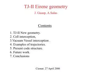
TJ-II Eirene geometry J. Guasp, A.Salas Contents 1. TJ-II New geometry. 2. Cell interception, 3.Vacuum Vessel interception . 4. Examples of trajectories. 5. Present code structure. 6. Future work. 7. Conclusions Ciemat. 27 April 2006 1. TJ-II New geometry

TJ-II Eirene geometry J. Guasp, A.Salas
E N D
Presentation Transcript
TJ-II Eirene geometry J. Guasp, A.Salas Contents 1. TJ-II New geometry. 2. Cell interception, 3.Vacuum Vessel interception . 4. Examples of trajectories. 5. Present code structure. 6. Future work. 7. Conclusions Ciemat. 27 April 2006
1. TJ-II New geometry An alternative geometry module for the application of Eirene to TJ-II has been built that avoids the problems of cell intersection, re-entry and holes that appear in other TJ-II models and simplifies at maximum the cell location and the intersection with the cell walls and other intercepting surfaces (Vacuum Vessel, limiters, etc.) that is the main time consuming task in the code. In this new model all the cells are hexahedra (6 plane faces, 8 vertex), two of the faces lie on toroidal planes and are square (but are not parallel), the two lateral faces are rectangles whose arists are horizontal or vertical while the upper and lower faces are quadrilateral (trapezoids) lying on an horizontal plane. The plasma is divided in toroidal layers (usually 38 by semiperiod, one octant, DF=1.2º) and in each layer an uniform cartesian grid, centered at the local magnetic axis position for the middle toroidal plane of the layer, is drawn. The grid extends both sides of the magnetic axis (the center) until the last node lies more than 5 cells outside the plasma. Usually there are, at maximum, 35 cells along the horizontal and vertical directions (DR , DZ~2 cm) The geometry is built only once for each magnetic configuration, outside Eirene, and is kept permanently as a binary file (44 Gby, ~5 min., program grideir).
F F F F F . . axis Y Z X . Z R 1. TJ-II New geometry axis The cells are built starting from the middle toroidal plane and launching horizontal lines normal to that plane until they intercept the near and rear toroidal planes. These intersections determine the cell vertex. By construction the cell walls are contiguous without neither holes nor overlapping.
1. TJ-II New geometry Drawing not very correct !!! . . o . x o Z R The cells are built starting from the middle toroidal plane and launching horizontal lines normal to that plane until they intercept the near and rear toroidal planes. These intersections determine the cell vertex.
1. TJ-II New geometry Central cells Red: Plasma Blue: Completelly inside the VV Orange:Some corner outside, Center inside Black crosses: Some corner outside. Center outside. Black Asterisk: All the cell outside the VV Vacuum cells Black X: Some corner inside. Center outside Blue X. Fully outside 100_44_64 Cell distribution at F= 0.6º (RA1) for the TJ-II geometry. View at the center of the 1st toroidal layer. Toroidal projection (R-R0, Z). 35x35 cells, at maximum, in each cross section (1.9 cm), 38 layers by semiperiod (1.2º). 91 poloidal vertex in VV (4º). Ports of VV eliminated farther than 50 cm from coil center.
1. H detection chords Chord dz(cm) smin 1 0.64 0.89 2 1.95 0.76 3 3.27 0.69 4 4.59 0.57 5 5.91 0.48 6 7.23 0.39 7 8.55 0.27 8 9.86 0.18 9 11.2 0.11 10 12.5 0.08 11 13.8 0.0 __________________________ 12 ----- 0.0 13 ----- 0.14 Toroidal cut at = -155º showing the plasma cross section, the 2nd limiter and the projection of the 1st chord, the closest point to the magnetic axis has s = 0.90 and is very near the limiter position. There are in total 11 chords, sharing a common origin, that are on the same vertical plane. The closest plasma radius reached by these chords appears in the table above and goes from 0.9 (1st) up to the axis (11th).
1. TJ-II New geometry Physical input variables (densities, temperatures, magnetic field, average plasma radius, etc.) are assigned to the cell centers. In addition a short series of codified labels are also associated to the cells, indicating the position of corners and center with respect to the Vacuum Vessel (VV), if they correspond either to the inside of the plasma, the border or the Scrape-off Layer (SOL), etc. Each of these cells (called central cells, cf. §3) has an associated number and also a label that says in which toroidal layer as well as horizontal and vertical cell is placed. Even if the geometry file is limited to a single octant, the Eirene calculations can be done (if so wished) for the full TJ-II 4 periods in order to deal with aperiodic scenarios. The real geometry seen by Eirene is the multiplication of the contained in the file after applying the Stellarator symmetry. For this reason each cell has a double identification: the one corresponding to the full 4 period geometry and the equivalent cell of the 1st octant.
1. TJ-II New geometry Central cells Red: Plasma Blue: Completelly inside the VV Orange:Some corner outside, Center inside Black crosses: Some corner outside. Center outside. Black Asterix: All the cell outside the VV Vacuum cells Black X: Some corner inside. Center outside Blue X. Fully outside 100_44_64 Cell distribution for the TJ-II geometry. Vertical projection (X, Y), ortogonal view from top. 35x35 cells, at maximum, in each cross section (2.0 cm). 38 layers by semiperiod (1.2º). 91 poloidal vertex in VV (4º). Ports eliminated farther than 50 cm from center.
1. TJ-II New geometry Central cells Red: Plasma Blue: Completelly inside the VV Orange:Some corner outside, Center inside Black crosses: Some corner outside. Center outside. Black Asterix: All the cell outside the VV Vacuum cells Black X: Some corner inside. Center outside Blue X. Fully outside 100_44_64 Cell distribution for the TJ-II geometry. Lateral projection (F, Z), ortogonal view from outside. 35x35 cells, at maximum, in each cross section (2.0 cm). 38 layers by semiperiod (1.2º), 91 poloidal vertex in VV (4º). Ports eliminated farther than 50 cm from center.
2. Cell interception As the cell grid is uniform in all coordinates, it is very easy given a point in space to know to which cell corresponds, even in the full 4 period case. The interception with the cell walls is also very easy and quick, it is enough to calculate the distance from a point inside the cell to the planes that limit it and are ahead in the velocity direction. As all the planes are either horizontal, vertical or toroidal the normal vectors to these faces are trivial and a very simple analytical formula can be applied. As, in addition, all the cells are concave from the inside there is certainty the the first intersection correponds to the minimum calculated distance, without need to do any residual or area sum checking.
2. Cell interception d = ([PV - P0] . n) / (n . v) Pf = P0 + d .v Pv n Pf Rear v P0 Front Example of intersection with the call walls. As the cells are concave from the inside, there is certainty the the first intersection correponds to the minimum calculated distance, without need to do any residual or area sum checking.
3. Vacuum Vessel interception The Vacuum Vessel (VV) of TJ-II has not been modelled in our geometry by volume cells, but as a mosaic of triangular plane plates. It forms always integral part of the geometry file. The starting point for this element was a VV CAD model (as with the plasma a single octant is enough) that later has been divided in uniform toroidal sections (just the same number as before: 39, DF = 1.2º), and each toroidal section in 90 pieces along the poloidal direction (DQ=4º). These rectangular, non planar, (sometimes extremely non planar) pieces were afterwards, divided consistently in 2 contiguous triangles. The triangle vertex list, as well as the normal vector of each triangle, are written into the geometry file. The origin (0º) of the poloidal direction is chosen starting from the helix described by the toroidal coil centers and along a radial horizontal line going to the inside of the torus. The poloidal angle goes in counter clock wise direction. In order to discard unnecessary complexity and useless space, before that depiecing, the VV was stripped of part of the ports. Anything lying farther than 50 cm from the coil center was ignored.
3. Vacuum Vessel interception In order to be able to determine when a trajectory intersects the VV a supplementary set of cells (called, perhaps not very properly, Vacuum cells) has been added to the geometry. It consists, for each toroidal layer, in a ring of 8 wide rectangular cells that surrounds completely the central cells. The inner walls of these new cells are in contact with the outer central layer. The more external walls are chosen so as they are fully outside the VV. So every point of the VV lies with certainty either inside these Vacuum cells or (i.e. the Hard Core points) somewhere in the central region. Further than these Vacuum cells there is only the Outside Darkness, any point lying there corresponds to an illegal cell, and when checked (i.e. by function LEAUSR) gives a negative cell number. This helps to determine if the intersection has happened: if a trayectory coming from a cell inside the VV goes either to a cell (central or not) where all the corners are outside the VV or it falls in the Darkness, it is a clear indication that, somewhere along the path, the VV has been hit, and this puts limits to the region where it is to be found.
3. Vacuum Vessel interception This finding is done in the following way. The more extreme coordinates of the intersecting trajectory are calculated, and for security measurements they are increased, along every direction, by a finite quantity (usually 10 times the size of a central cell). Inside this region all the VV triangles are checked, first calculating the distance to the initial point but, as the VV can be as well concave as convex from the inside (and sometimes extremely convex), we can not, anymore, take the nearest triangle, as was done for the central cells. Instead, this time, we must be sure that the point of intersection with the plane of the triangle is really inside that triangle. This check is done by an sum of areas algorithm, that is the equivalent of the residualtheorem in complex variable, when applied to a triangular contour. If the point is inside, then the sum of the areas subtended by the point and each couple of vertex must be just equal to the triangle area. In the contrary the point is outside. Of course allowance must be given for the finite accuracy of the computer.
P1 n Pv F v P0 3. Vacuum Vessel interception Incorrect drawing !! d = ([PV - P0] . n) / (n . v) Pf = P0 + d .v Example of intersection with the VV: For every one of the triangles placed inside the extreme limits of the detection zone (increased by some security margins), a sum of areas algorithm must be performed, and only if the check is affirmative the point retained as the exit one.
P 3 . 1 P 1 2 3 1 . P 2 3. Vacuum Vessel interception . 3 2 ¡¡¡ Plane Geometry!!! In the Sum of Areas algorithm, if point P is inside the triangle (123) then: AP12 + AP23 + AP31 = A123 Otherwise if P is outside: AP12 + AP23 + AP31 > A123 And it is enough than anyone of the partial areas AP12, etc. be > A123 to be sure that the point is outside the triangle.
4 Examples of trajectories In this way the neutral trajectories can be followed The next figures show two different examples of trajectories, both correspond to a He case, where the neutrals are born at the vacuum vessel surface and, usually, are absorbed at the plasma and reflected many times at the VV. Each point corresponds to either a cell interception of a VV reflexion The first couple correspond to an unusually short trajectory, and therefore can be visualised much better, under a vertical and a lateral view. The second couple is a more usual one, 261 points, this is the usual number of interceptions and reflections before the particle is absorbed.
4 Examples of trajectories A very very short trajectory for an He atom. Vertical projection (X, Y). It starts in the green square an finish, by ionisation, near the plasma center (red losange).
4 Examples of trajectories A very very short trajectory for an He atom. Lateral projection (, Z). It starts in the green square an finish, by ionisation, near the plasma center (red losange).
4 Examples of trajectories A more usual trajectory for an He atom (261 points). Vertical projection (X, Y). It starts in the green square (first cuadrant near the wall) an finish, by ionisation, near the plasma center (red losange, lower 4th cuadrant).
4 Examples of trajectories 261 A more usual trajectory for an He atom (261 points). Vertical projection (F, Z) It starts in the green square (right middle) an finish, by ionisation, near the plasma center (red losange, left middle).
5. Present code structure The 2004 version of Eirene has been installed in the two parallel computers of Ciemat and is running properly: jen50: SGI Origin-3800 with a f90 MIPSpro compiler version 7.41, and 124 processors fénix: SGI Altix-3700 with the f90 INTEL compiler version 8.0, and 96 PE's In both computers the code has been compiled with optimisation -O2/3 and runs in parallel under MPI. The code itself runs after a preparatory program preproc, serial, very fast that makes many things: reads and checks the geometry, reads the files containing the plasma input profiles, or alternatively extracts them for the TJ-II discharge Data Base, reads data for the diagnostic chords and generates the corresponding cartesian coordinates expected by Eirene and, mainly, modifies and prepare the input file. In the same way, after Eirene exits, a second serial program postproc is executed, it reads several files created by Eirene (i. e. the detailed tallies results from PRTTAL that have been diverted, at Ciemat, to files, etc.) and prints several kind of results or generates files for graphic representation.
Eirene Initialisation Trajectory calculation Gathering of data and results 5. Present code structure Geometry Preliminay input file for Eirene Namelist (modalities, chords, etc.) Radial plasma profiles Preproc Graphic files Main results: (neutral distribution in plasma, ibid. along chords, etc.) Postproc
5. Present code structure The TJ-II helical geometry has been adapted to Eirene using the options: LEVGEO = 6 (general geometry), INDPRO = 12*5 (calls to PROUSR for the input plasma profiles) and SORLIM < 0. (calls to SAMUSR for the source distribution). In the present version for TJ-II there are up to 19 non standard surfaces: 1. The Vacuum Vessel. Reflecting. 2. The limbo. Absorbing. Used to finish pathological trajectories (~ 10-5) 3. The plasma border. Transparent 4.- 5. Two limiters. Reflecting. 6.- 7. Two gas puffing valves. Transparent. Included to allow these sources. 8.- 19. 4 NBI injectors. Included as sources. And 4 Pump valves. Usually there are up to 13 sources. (7 in jen50 due to some unfathomable errors) 1. The VV wall. 2.- 3. The two limiters 4.- 5. The two gas puffing valves. 6.- 13. The 4 NBI injectors and 4 Pumps. In reason of a parallelisation problem we can use now only a single stratum for all the sources distributed in up to 12(7) substrata. Although a palliative has been found.
5. Present code structure Execution times at fenix computer (with diagnostic chords): Case He: 9.5x10⁶ trajectories, total time = 12 min. (24 PEs, Batch) Case H: 2.4x10⁶ trajectories, total time = 8 min. (24 PEs, Batch) These execution times are approx. double at Jen50 computer.
5. Present code structure Many of the results that previously did appear on the output file have been diverted to files that can be read by other programs (i.e. postproc, vertray, verflux, etc.). The main results that can be obtained now are the following: Resulting electron density radial profiles Distribution of neutral particles in the plasma, averaged over magnetic surfaces. Distribution of neutral particles along selected TJ-II and diagnostic chords CX Energy spectra along selected TJ-II chords. Halpha emissivity along selected TJ-II chords. All those results allow the possibility for plotting Plots for trajectories ( < 15000, < 1000 points by trajectory). Program vertray. Also included: Emissivity of 4 He lines (similar to sigha.f and halpha.f) along chords. Distribution of impacts on the VV and the plasma surface (too much disk space consuming … …). Program verflux. Driver to allow parameter scans. Driver to allow parameter fits to experimental data.
5. Present code structure tp = 13 ms tp = 13, 13, 17 ms Radial profiles of the neutral density in the plasma, averaged over magnetic surfaces. Near the plasma border the exponential fitting separates visibly from the calculations. The absolute values of these densities are inversely proportional to the supposed particle confinement time (tp).
5. Present code structure tp = 13 ms tp = 13 ms Longitudinal profile of neutral density along two chords of TJ-II.
6. Supplementary work Already done: Emissivity of 4 He lines (similar to sigha.f and halpha.f) along chords. Distribution of impacts on the VV and the plasma surface (too much disk space consuming … …). Program verflux. Driver to allow parameter scans. Driver to allow parameter fits to experimental data. Comparison of Eirene results with the experimental emissivity of He spectral lines. Partially done: Determination of the neutral distribution near the limiters by means of H signals. In preparation: Determination of the neutral distribution inside the plasma by means of CX signals. Explore the possibility to use the H signals present in the Scattering Thomson measurements. Etc., etc.
7. Conclusions An alternative geometry module for the application of Eirene to TJ-II has been built that avoids the problems of cell intersection, re-entry and holes, and simplifies at maximum the cell location ant the intersection with the cell walls and other intercepting surfaces (Vacuum Vessel, limiters, etc.) that is the main time consuming task in the code. Efficient algorithms for the interception of the trajectories with cell walls and the TJ-II Vacuum Vessel have been incorporated. The geometry has been adapted to the 2004 Eirene version and is now working satisfactorily in the two parallel computers of Ciemat. Comparison with experimental data of He spectral line emission and H has been adressed also.