Computer Simulation
Computer Simulation. The Essence of Computer Simulation. A stochastic system is a system that evolves over time according to one or more probability distributions.

Computer Simulation
E N D
Presentation Transcript
The Essence of Computer Simulation • A stochastic system is a system that evolves over time according to one or more probability distributions. • Computer simulation imitates the operation of such a system by using the corresponding probability distributions to randomly generate the various events that occur in the system. • Rather than literally operating a physical system, the computer just records the occurrences of the simulated events and the resulting performance of the system. • Computer simulation is typically used when the stochastic system ivolved is too complex to be analyzed satisfactorily by analytical models. 12-2
Example 1: A Coin-Flipping Game • Rules of the game: • Each play of the game involves repeatedly flipping an unbiased coin until the difference between the number of heads and tails tossed is three. • To play the game, you are required to pay $1 for each flip of the coin. You are not allowed to quit during the play of a game. • You receive $8 at the end of each play of the game. • Examples: 12-3
Computer Simulation of Coin-Flipping Game • A computer cannot flip coins. Instead it generates a sequence of random numbers. • A number is a random number between 0 and 1 if it has been generated in such a way that every possible number within the interval has an equal chance of occurring. • An easy way to generate random numbers is to use the RAND() function in Excel. • To simulate the flip of a coin, let half the possible random numbers correspond to heads and the other half to tails. • 0.0000 to 0.4999 correspond to heads. • 0.5000 to 0.9999 correspond to tails. 12-4
Freddie the Newsboy • Freddie runs a newsstand in a prominent downtown location of a major city. • Freddie sells a variety of newspapers and magazines. The most expensive of the newspapers is the Financial Journal. • Cost data for the Financial Journal: • Freddie pays $1.50 per copy delivered. • Freddie charges $2.50 per copy. • Freddie’s refund is $0.50 per unsold copy. • Sales data for the Financial Journal: • Freddie sells anywhere between 40 and 70 copies a day. • The frequency of the numbers between 40 and 70 are roughly equal. 13-8
Application of Crystal Ball • Four steps must be taken to use Crystal Ball on a spreadsheet model: • Define the random input cells. • Define the output cells to forecast. • Set the run preferences. • Run the simulation. 13-10
Step 1: Define the Random Input Cells • A random input cell is an input cell that has a random value. • An assumed probability distribution must be entered into the cell rather than a single number. • Crystal Ball refers to each such random input cell as an assumption cell. • Procedure to define an assumption cell: • Select the cell by clicking on it. • If the cell does not already contain a value, enter any number into the cell. • Click on the Define Assumption button. • Select a probability distribution from the Distribution Gallery. • Click OK to bring up the dialogue box for the selected distribution. • Use the dialogue box to enter parameters for the distribution (preferably referring to cells on the spreadsheet that contain these parameters). • Click on OK. 13-11
Step 2: Define the Output Cells to Forecast • Crystal Ball refers to the output of a computer simulation as a forecast, since it is forecasting the underlying probability distribution when it is in operation. • Each output cell that is being used to forecast a measure of performance is referred to as a forecast cell. • Procedure for defining a forecast cell: • Select the cell. • Click on the Define Forecast button on the Crystal Ball tab or toolbar, which brings up the Define Forecast dialogue box. • This dialogue box can be used to define a name and (optionally) units for the forecast cell. • Click on OK. 13-14
Step 3: Set the Run Preferences • Setting run preferences refers to such things as choosing the number of trials to run and deciding on other options regarding how to perform the simulation. • This step begins by clicking on the Run Preferences button on the Crystal Ball tab or toolbar. • The Run Preferences dialogue box has five tabs to set various types of options. • The Trials tab allows you to specify the maximum number of trials to run for the computer simulation. 13-16
Step #4: Run the Simulation • To begin running the simulation, click on the Start Simulation button. • Once started, a forecast window displays the results of the computer simulation as it runs. • The following can be obtained by choosing the corresponding option under the View menu in the forecast window display: • Frequency chart • Statistics table • Percentiles table • Cumulative chart • Reverse cumulative chart 13-18
Choosing the Right Distribution • A continuous distribution is used if any values are possible, including both integer and fractional numbers, over the entire range of possible values. • A discrete distribution is used if only certain specific values (e.g., only some integer values) are possible. • However, if the only possible values are integer numbers over a relatively broad range, a continuous distribution may be used as an approximation by rounding any fractional value to the nearest integer. 13-19
A Popular Central-Tendency Distribution: Normal • Some value most likely (the mean) • Values close to mean more likely • Symmetric (as likely above as below mean) • Extreme values possible, but rare 13-20
The Uniform Distribution • Fixed minimum and maximum value • All values equally likely 13-21
The Discrete Uniform Distribution • Fixed minimum and maximum value • All integer values equally likely 13-22
A Distribution for Random Events: Exponential • Widely used to describe time between random events (e.g., time between arrivals) • Events are independent • Rate = average number of events per unit time (e.g., arrivals per hour) 13-23
Yes-No Distribution • Describes whether an event occurs or not • Two possible outcomes: 1 (Yes) or 0 (No) 13-24
Distribution for Number of Times an Event Occurs: Binomial • Describes number of times an event occurs in a fixed number of trials (e.g., number of heads in 10 flips of a coin) • For each trial, only two outcomes are possible • Trials independent • Probability remains the same for each trial 13-25