Performance Improvement in PaaS
1.03k likes | 1.23k Vues
Performance Improvement in PaaS. Group I. Improving Performance of systems in PaaS. The PaaS system is not always easy to define, but with the increasing use of cloud services it has fueled our need for improving performance.

Performance Improvement in PaaS
E N D
Presentation Transcript
Performance Improvement in PaaS Group I
Improving Performance of systems in PaaS The PaaS system is not always easy to define, but with the increasing use of cloud services it has fueled our need for improving performance. We will look at two areas in the PaaS platform and how to evaluative there performance, Map/Reduce and HDFS.
Presentation Order • First there will be a intro into Time Series Analysis. This is to get a feel for what it is and how we can use it to improve performance in systems. • Next we will look at WEKA, a very common and well know application for Time Series Analysis. • After introducing the tools to help with evaluation we will look at HDFS and improving small file I/O performance. • Finishing up we look at MapReducePerformance in Heterogeneous Hadoop Clusters
Presenters Time Series Analysis Katrina Christopher Time Series Analysis and forecasting using WEKA JoysonJacob Implementing WebGIS on Hadoop: A Case Study of Improving Small File I/O Performance on HDFS Marc DelaCruz Improving MapReduce Performance in Heterogeneous Hadoop Clusters Roshan Muralidharan
Time Series Analysis By Katrina Christopher
What is Time Series Analysis Time series analysis is a process of using statistical techniques to model and explain a time-dependent series of data points. • In other words, we are studying data that is dependent on random variables (or vectors) as appose to studying the dependence of one variable on another. • We use time series models to help us generate future observations based on what we have seen.
Some areas that often use Time Series Analysis • Gain a better understanding of the data • Predict future values • Optimally control systems • Monitor processes • Derive computer simulations • Prepare countermeasures in cases of unexpected events • Improve output, quality and/or performance of a system
Characteristics of time series data • Data is not generated independently • Its dispersion varies in time • The data is often governed by a trend • It has cyclic components
Objective The main objective of time series analysis Visualizing – Looking at the data with plots, graphs and other plotters. Filtering – Used in preprocessing to smooth things out. Prediction – Applying the Stochastic Models.
Visualizing Plotting, graphs and other techniques can give you a better look at the data. These graphs and plots can help the user make simple measurements and identify existing tends, seasonality, turning points…ect.
Two different types of analysis When looking at time series there are two main types of analysis • Time Domain Analysis is used to predict the probability of future values by analyzing data over a time period. • Frequency Doman Analysis studies the cycle and their frequency within the time series. Used in preprocessing.
Smoothing Techniques Smoothing techniques are used to reduce irregularities (random fluctuations) in time series data. This preprocessing helps separate the behavior of a time series into trend vs. cyclical and irregular components. Studying the data can show hidden cycles and their relative strengths
Prediction Given an observed time series, a typical aim is to predict future values. This is based on the principle that the behavior of the occurrence in the the past is also maintained in the future.
TimeDomain • Time domain generally uses a stochastic model to help predict future values in terms of some probability distribution. • Given a set of observed time series, how do you forecast future values. • Find a model that best describes the evolution of the observed “time series” over time • Fit this model to the data. • Forecast based on the fitted model
The Stochastic class of models We can break these up into two classes of models, those that are stationary and those that are non-stationary. • Stationary models assume that the process remains in equilibrium about a constant mean value ARMA (Autoregressive Moving Average) which is broken up into two parts • AR(Autoregressive) • MA(Moving Average) • Non-stationary models describe data that have no mean constant level over time which are ARIMA (Autoregressive Integrated Moving Average)
ARMA Model and ARIMA ARMA/ARIMA • These models are the most basic time series model and can be fit with many major statistical packages. • This the tool for understanding and perhaps, predicting future values. • The disadvantage is that it is often not very descriptive of the underlying processes, the parameters are difficult to interpret.
Reference • http://en.wikipedia.org/wiki/Weka_(machine_learning) • http://en.wikipedia.org/wiki/RapidMiner • http://cran.r-project.org/doc/contrib/Ricci-refcard-ts.pdf • http://www.stat.berkeley.edu/~aditya/Site/Statistics_153;_Spring_2012_files/Lecture%20One.pdf • MargheritaGerolimetto,“Introduction to time series analysis”, November 3, 2010 • http://home.ubalt.edu/ntsbarsh/stat-data/forecast.htm#rsodasp • H. Kosorus, J. Honigl, J. Kung, “Using R, WEKA and RapidMiner in time series analysis of sensor data forstructuralhealthmonitoring,” WorkshoponDatabase and ExpertSystemsApplications, Aug-Sep 2011, pp. 306-310
Time Series Analysis and forecasting using WEKA By Joyson Jacob
Time Series Forecasting • Process of using a model to generate predictions for future events based on known past events. • E.g.: capacity planning, inventory replenishment, sales forecasting and future staffing levels.
WEKA • A popular suite of machine learning software written in Java. • Contains a collection of machine learning algorithms for data mining tasks. • Contains tools for data pre-processing, classification, regression, clustering, association rules, and visualization. • Weka allows forecasting models to be developed, evaluated and visualized. • Provides a time series forecasting environment for Weka.
Time Series Analysis in Weka • The framework takes a machine learning/data mining approach to modeling time series. • The environment takes the form of a plugin tab in Weka's graphical "Explorer" user interface. • Transforms the data into a form that standard propositional learning algorithms can process. • By default, the time series environment is configured to learn a linear model, i.e. a linear support vector machine. • Includes both command-line and GUI user interfaces
Forecasting steps • Remove temporal ordering of individual input examples by encoding the time dependency via additional input fields. • Various other fields also computed automatically to allow the algorithms to model trends and seasonality. • Any of Weka's regression algorithms are then applied to learn a model. E.g. multiple linear regression. • This model is then used to generate forecasts.
Using the environment • After installing, time series modeling environment is a new tab in Weka's Explorer GUI
Basic Configuration Parameters 1. Number of time units to forecast • controls how many time steps into the future the forecaster will produce predictions for. • default is set to 1 2. Time Stamp • allows the user to select which, if any, field in the data holds the time stamp • If there is a date field in the data then selected automatically. • Else the "<Use an artificial time index>" option is selected. • User may select the time stamp manually (E.g. non-date numeric field)
Basic Configuration Parameters 3. Periodicity • allows the user to specify the Periodicity of the data. • used to set reasonable defaults for the creation of lagged variables • If a date field has been selected as the time stamp, then the system automatically detects the periodicity. • Else the user can tell the system what the periodicity is. 4. Skip List • allows the user to specify time periods that should not count as a time stamp increment with respect to the modeling, forecasting and visualization process. • E.g. "weekend", "sat", "Tuesday", “2011-07-04”, etc.
Basic Configuration Parameters 5. Confidence Intervals • user can opt to have the system compute confidence bounds on the predictions that it makes. • default confidence level is 95% • all the one-step-ahead predictions on the training data are used to compute the one-step-ahead confidence interval. 6. Perform Evaluation • system performs an evaluation of the forecaster using the training data. • Once the forecaster has been trained on the data, it is then applied to make a forecast at each time point (in order) by stepping through the data.
Output • Forecasting model • Forecasted values in text form and a textual description of the model learned. E.g.: the model learned on the airline data.
Output 2. Training evaluation
Output 3. Graphs of forecasted values beyond the end of the training data
Advanced Configuration Features • Gives the user full control over a number of aspects of the forecasting analysis including the underlying model learnt. • Each of these has a dedicated sub-panel in the advanced configuration panel. These include: 1. Base Lerner • provides control over which Weka learning algorithm is used to model the time series. • the choice of underlying model and parameters • Default is to use a linear support vector machine for regression
Advanced Configuration 2. Lag Creation • Lagged variables are the main mechanism by which the relationship between past and current values of a series can be captured by propositional learning algorithms. • They create a "window" or "snapshot" over a time period. • E.g. if you had hourly data, you might want lags up to 24 time steps or 12 steps. 3. Periodic attributes • allows the user to customize which date-derived periodic attributes are created • E.g. if the data has a monthly time interval then month of the year isautomatically included as variables in the data.
Advanced Configuration 4. Overlay data • "overlay" data: input fields that are to be considered external to the data transformation and closed-loop forecasting processes. • i.e. data that is not to be forecasted, can't be derived automatically and will be supplied for the future time periods to be forecasted. • This makes it possible for the model to take into account special historical conditions (e.g. stock market crash) and factor in conditions that will occur at known points in the future. • The default is not to use overlay data.
Advanced Configuration 5. Evaluation • allows the user to select which evaluation metrics they wish to see • give an indication of how the well forecaster's predictions are doing compared to just using the last known target value as the prediction. • Can configure whether to evaluate using the training data and/or a set of data held out from the end of the training data. • Same as selecting Perform evaluation in the Basic configuration • By default, the mean absolute error (MAE) and root mean square error (RMSE) of the predictions are computed. Other available metrics are: • Mean absolute error (MAE) • Mean squared error (MSE), etc.
References • http://en.wikipedia.org/wiki/Weka_%28machine_learning%29 • http://www.cs.waikato.ac.nz/~ml/weka/ • http://wiki.pentaho.com/display/DATAMINING/Time+Series+Analysis+and+Forecasting+with+Weka
Implementing WebGIS on Hadoop: A Case Study of Improving Small File I/O Performance on HDFS By Marc DelaCruz
Introduction • The paper discusses using Hadoop to support WebGIS applications • WebGIS stands for Web Geographic Information System (GIS). • GIS is built for acquisition, storage, management of spatial data and attributes • It provides users ability to access, manage, and share global geographic data. • The paper proposes to optimize I/O performance of small files on HDFS 2
Introduction • The paper proposes to optimize I/O performance of small files on HDFS • The idea is to combine small files into large ones to reduce the file number and build an index for each file • WebGIS access patterns are taken into account • Results show that • execution time of reading and storing files are improved significantly • Memory usage rate decreases several times 3
Motivation • HDFS was originally designed to manage large file, not for small files • HDFS has performance penalty when managing a large amount of small files • Example: • 550,000 small files of 1KB to 10KB size • Unacceptable execution time: takes 7.7 hours to store into HDFS vs 660 seconds on local file system • High memory usage rate: 63.53% occupied during storing operation 4
Motivation • Why so slow? • HDFS stores files with metadata and has several replicas (3 copies by default) • Metadata management is time-consuming • For small files, most time is spent managing metadata, less time on data-transfer • Small files increase overhead • Metadata are kept in name node while chunk's info are kept in data nodes • Both chunks and metadata are stored in physical memory 5
WebGIS File Access Patterns • Some metadata attributes are same • e.g. file owner, access permissions • Some attributes are not important and can be ignored • e.g. created time and modified date • WebGIS provides map-browsing interface for clients • Geographically proximal images are likely accessed later • Several latest versions of data need to be reserved during updates 6
Approach • Idea: merge small files into big ones and build an index for each small file using hash index • First, files are grouped and stored consecutively in physical memory by geographic locations • Second, historical spatial data are stored in several versions. Versions are reserved during updating • Files < 16MB are considered small files 7
File Grouping • Files are organized as small tiles 256x256 pixels • Location info are represented by directories and file name • Position is dictated by 3 variables: (L, (x,y)) • L is the scale level from 0 - 17 • x and y are coordinates of X axis and Y axis respectively 9
File Grouping • Grouping schema combines n x n files which are adjacent in locations • n is application specific but must be powers of 2 • The file at the up-left is defined as the first file • Given a tile of (L, (x,y)), the first file is computed as: 10
Index File • Index file has two parts: • index header, and • index data block 11
Index File • Index Header • Number of Buckets x Factor decides maximum number of indexed files • if file number exceeds this value, the Number of Buckets should be increased and all hash values are recalculated • Number of Buckets must be big enough to avoid recalculation 12
Index File • Index Data Block
Index File • Index Data Block • UFLAG: used flag; says whether block is in use • VFLAG: valid flag; indicates validity, zero when index data is deleted • Key Length: valid length of the key of the index of the block • Key Field: the actual key with max length of 128 bytes • File Block: serial number of data file in w/c the file is stored (positive means its valid) • The index data block may contain more than one value for multiple versions 14
Data File • Data Files also have 2 parts: • Data Header, and • Data Block 15
Data File • Data Header • Number of Files: records the total number of files in this data file • Number of Valid Files: valid files in this data file • Both fields increase when a file is added • When deleting files, Number of Valid Files decreases but Number of Files is unchanged 16