MACHINE LEARNING

1. MACHINE LEARNING

2. Marc Chagall

3. (Vincent van Gogh)

4. Marc Chagall ? Or Vincent van Gogh?

5. (Paul Gaugin)

6. (Vincent van Gogh)

7. Gaugin or Van Gogh?

8. Induction vs Deduction • Deductive reasoning is the process of reasoning from one or more general statements (premises) to reach a logically certain conclusion. • Inductive is reasoning in which the premises seek to supply strong evidence for (not absolute proof of) the truth of the conclusion.

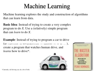
9. MACHINE LEARNING • The human mind is the best pattern recognizer and classifier, can recognize pattern in spite of noise and vagueness. • 1. The human mind learns by induction • 2. The human mind recognizes looking at the whole and not at individual parts.

10. Learning is a fundamental and essential characteristic of biological neural networks. The ease with which they can learn led to attempts to emulate a biological neural network in a computer.

11. How does human mind learn? • A neuron consists of a cell body, soma, a number of fibers called dendrites, and a single long fiber called the axon. • The human brain incorporates nearly 10 billion neurons and 60 trillion connections, synapses, between them. By using multiple neurons simultaneously, the brain can perform its functions much faster than the fastest computers in existence today.

12. Human Learning: Key features Human beings learn patterns by induction (seeing examples) The knowledge acquired remains in their memory, The knowledge is recalled when required to recognize a pattern not seen before

13. Machines Learning : Key features • Show the computer several examples of a pattern repeatedly. • Hope that it would learn the “diagnostic” characteristic of the pattern. • We make sure that the computer has learnt adequately (how?) • The knowledge acquired by the computer will remains in their “memory” (how?) • The computer will recall the knowledge when asked to classify an unseen pattern

14. MACHINE LEARNING • The human mind is much better than a computer at recognizing vague/noisy patterns - • A well-trained computer can process larger amount of information! • Non-linear model –same feature gets different weights in different combinations

15. MACHINE LEARNING • Downside – the computer will not tell you why it has classified a particular pattern in a particular way. • A blackbox!! • Like human mind!!

16. Problems with Probabilistic/Fuzzy methods Weights of Evidence Correlation between maps Fuzzy Logic Subjective judgment -> difficult to reproduce

17. MACHINE LEARNING • Neural netwroks • Hybrid Neurofuzzy systems • Bayesian Classifier • Genetic Algorithms • SOM

18. 2 1 2 1 3 1 2 4 3 3 3 4 5 5 5 4 Unique Condition No Predictor patterns Class – Potential (1) or not potential (0) Slope Drainage density Soil permeability Distance from permeable struct 1 >60 1 - 2 10000 5 ?? 2 45 - 60 2 - 3 5000 2. ?? 3 30 - 45 3 - 4 12500 3 ?? 4 15 - 30 4 - 5 1000 4. ?? 5 <15 0 - 1 25000 1. ?? MACHINE LEARNING • Resource potential modelingcan be viewed as a pattern recognition problem. • Involves predictive classification of each spatial unit characterized by a unique combination of spatially coincident predictor patterns (or unique conditions) as mineralized or barren with respect to the target mineral deposit-type. In machine learning jargon, its called a feature vector Study area Unique conditions grid map GIS Overlay

19. Attribute1(i), Attribute2(i), …………., Attribute6(i) 0 Attribute1(i), Attribute2(iii), …………., Attribute6(iv) 1 Attribute1(ii), Attribute2(i), …………., Attribute6(v) 1 Attribute1(v), Attribute2(i), …………., Attribute6(i) 0 … … Attribute1(iii), Attribute2(ii), …………., Attribute6(vi) 1 MACHINE LEARNING

20. UNIQUE CONDITIONS GRID

21. Converting GIS layers to feature vectors target GIS raster layers output Input feature vector [3, 8, 33, 800] 1 SiO2 content Rock type Fe content Distance to Fault 1 0 0 0 0 0 0 0 0 0 0 0 1 1 0 0 0 0 0 0 Deposits

22. Backpropagation Input Vector Actual Output (y) SiO2 content 40 MgO content 11 NN 0.36 Fe content 20 Distance to Fault 600 Error = (d – y) 0.64 Deposits Targeted Output (d) =1 Deposits Feed forward

23. Inside the black-box………….??? A neuron (Nodes) (processing units) w11 fi w12 x11 fh w21 w22 fi fo x21 w31 fh fi w32 w41 w42 fi A layer of output neurons (Output layer - O) A Layers of input neurons (Input layer -I) A layer of Hidden neurons (Hidden layer -H) Neuron – Neural, but what is network? what is network? – Connect all neurons…..

24. An artificial neural network consists of a number of very simple processors, also called neurons, which are analogous to the biological neurons in the brain. • The neurons are connected by weighted links passing signals from one neuron to another. • The output signal is transmitted through the neuron’s outgoing connection. The outgoing connection splits into a number of branches that transmit the same signal. The outgoing branches terminate at the incoming connections of other neurons in the network.

25. Properties of architecture • No connections within a layer • No direct connections between input and output layers • Fully connected between layers • Often more than 3 layers • Number of output units need not equal number of input units • Number of hidden units per layer can be more or less than input or output units

26. Neuron functions (Also called Activation functions) • The neuron computes the weighted sum of the input signals and compares the result with a threshold value, . If the net input is less than the threshold, the neuron output is 0/–1. But if the net input is greater than or equal to the threshold, the neuron becomes activated and its output attains a value +1. • The neuron uses the following transfer or activationfunction:

27. Activation functions of a neuron Radial basis function

28. HIDDEN LAYER INPUT LAYER OUTPUTLAYER Error p1 w11 p2 ∫ Network output w21 Σ ∫ Σ . . y t . . Target output w2n w1n ∫ pn Σ – transfer function f – activation function

29. NETWORK PARAMETERS • Weights • Number of neurons • Function parameters NETWORK TRAINING Iterative modifications of network parameters to minimize error TRAINING SAMPLES (VALIDATION SAMPLE) - Feature vectors whose class is known

30. TRAINING ALGORITHM • Problem of assigning ‘credit’ or ‘blame’ to individual elements • involved in forming overall response of a learning system • (hidden units) • In neural networks, problem relates to deciding which weights • should be altered, by how much and in which direction. • Analogous to deciding how much a weight in an early layer contributes to the output and thus the error • We therefore want to find out how weight wij affects the error i.e. we want:

31. Backpropagation learning algorithm ‘BP’ ( Rumelhart, Hinton and Williams ,1986) BP has two phases: Forward pass phase: computes ‘functional signal’, feedforward propagation of input pattern signals through network Backward pass phase: computes ‘error signal’, propagates the error backwards through network starting at output units (where the error is the difference between actual and desired output values)

32. Backpropagation learning algorithm ‘BP’ ( Rumelhart, Hinton and Williams ,1986) Uses gradient descent (steepest descent) and Delta Rule for minimizing error Any given combination of weights will be associated with a particular error measure. The Delta Rule uses gradient descent learning to iteratively change network weights to minimize error (i.e., to locate the global minimum in the error surface).

33. Backpropagation learning algorithm ‘BP’ ( Rumelhart, Hinton and Williams ,1986) 0 To find a minimum of a function using gradient descent, one takes steps proportional to the negative of the gradient (or of the approximate gradient) of the function at the current point. If instead one takes steps proportional to the positive of the gradient, one approaches a maximum of that function; the procedure is then known as gradient ascent.

34. Backpropagation learning algorithm ‘BP’ ( Rumelhart, Hinton and Williams ,1986) Step size: Learning rate Too small steps, slow convergence of error, but convergence to minima assured Too big steps, fast convergence but minima may be missed

35. Backpropagation learning algorithm ‘BP’ ( Rumelhart, Hinton and Williams ,1986) Derivative: How a function changes as its input changes Or how much one quantity changes in response to a change in some other quantity for example, the derivative of the position of a moving object with respect to time is the object's instantaneous velocity. ≈ Slope/gradient Black: the graph of a function Red: tangent line to that function The slope/gradient of the tangent line is equal to the derivative of the function at the marked point. Black: Maximum Value White: Minimum value Gradient points to wards higher values

36. Backpropagation learning algorithm ‘BP’ ( Rumelhart, Hinton and Williams ,1986) Partial derivative: Suppose a function has several variables. Partial derivative of the function with respect to one of the variables is how the function changes as that variable changes (other variables assumed constant)

37. Backpropagation learning algorithm ‘BP’ ( Rumelhart, Hinton and Williams ,1986) In the context of Neural networks - Function: Error Variables: weights/function parameters Conceptual basis of weight adjustment: Determine partial derivative of error with respect to each of the weights/parameters Adjust each weight in a direction opposite to the steepest gradient

38. X1 X2 X3 X4 Input feature vector X Input layer I Hidden layer J Output layer K

39. Backpropagation learning algorithm ‘BP’ I J K Calculate errors of output neurons: δK= OK(1 - OK) (Target - OK) 2. Change output layer weights WJ_K= WJ_K + η*δK*OJ 3. Calculate (back-propagate) hidden layer errors δJ = OJ (1 – OJ) (δK *WJ_K) 4. Change hidden layer weights WI1_J= WI1_J+ η*δJ*x1 WI2_J= WI2_J+ η*δJ*x2 WI1_J I1 X1 WJ_K I2 WI2_J X2 Output layer Hidden layer Input layer The constant η (called the learning rate, and nominally equal to one) is put in to speed up or slow down the learning if required.

40. Data 2 hidden neurons 1 output neuron Learning rate 0.5 Sigma function Start with random weights between 0 and 1, Run the algorithm. See if the error is reduced in the next iteration.

41. Practical considerations: Neural Network training • Collect all possible examples of the pattern • Encode and format the data • Classify in three subset: • Training set (70%) • Validation(20%) • Testing set (10%) • Or use n-fold (k-fold) validation (also called jack-knifing) • GOLDEN RULE : Number of training set samples should be at least 3 times the number of parameters to be estimated –

42. Practical considerations: Neural Network training: Input data encoding and formatting

43. Practical considerations: Neural Network training: Input data encoding and formatting

44. Practical considerations: Neural Network training: Input data encoding and formatting

45. Practical considerations: Neural Network training: Input data encoding and formatting Training data Validation data Testing data

46. Practical considerations: Neural Network training: Training Chose a subset of training samples Computer the error for the subset Update weights so as to reduce the error (e.g., using gradient descent) Calculate error for validation samples The above 4 steps comprise one pass through the subset of training samples along with an updating of weights, called a “training epoch” Number of training samples in the subset is epoch size. You can use an epoch size of 1, or an epoch size of n (=number of training samples), or any size between 1 and n. Save the weights/parameters after every training epoch

47. Practical considerations: Neural Network training: Training Plot training and validation errors against number of training epochs Validation error minimizes at 70 epochs, beyond which it begins to rise => The weights/parameters saved after 70th epoch comprise the trained network

48. Practical considerations: Neural Network training: Training Before jumping to processing the samples to be classified, test your trained network with the testing samples (the third subset)

49. Optimization of the number of hidden neurons