Download
1 / 108
1.08k likes | 1.32k Vues
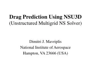
Results from the 3 rd Drag Prediction Workshop using the NSU3D Unstructured Mesh Solver. Dimitri J. Mavriplis University of Wyoming. Overview. Description of Meshes Description of NSU3D Solver Sample performance Preliminary Sensitivity Evaluations WB and WBF Results W1 and W2 Results

E N D
Results from the 3rd Drag Prediction Workshop using the NSU3D Unstructured Mesh Solver Dimitri J. Mavriplis University of Wyoming
Overview • Description of Meshes • Description of NSU3D Solver • Sample performance • Preliminary Sensitivity Evaluations • WB and WBF Results • W1 and W2 Results • Including runs performed at Cessna on 2nd family of grids • Conclusions
General Gridding Guidelines • Grid Convergence Cases: • DLR F6 WBF • 3 grid levels required • DLR F6 WB • Medium grid required, coarse/fine optional • Wing1 and Wing2 • Four grid levels required
General Gridding Guidelines • Grid Resolution Guidelines • BL Region • Y+ < 1.0, 2/3, 4/9, 8/27 (Coarse,Med,Fine,VeryFine) • 2 cell layers constant spacing at wall • Growth rates < 1.25 • Far Field: 100 chords • Local Spacings (Medium grid) • Chordwise: 0.1% chord at LE/TE • Spanwise spacing: 0.1% semispan at root/tip • Cell size on Fuselage nose, tail: 2.0% chord • Trailing edge base: • 8,12,16,24 cells across TE Base (Coarse,Med,Fine,Veryfine)
General Gridding Guidelines • Grid Convergence Sequence • Grid size to grow ~3X for each level refinement • 1.5X in each coordinate direction (structured) • Maintain same family of grids in sequence • Same relative resolution/topology/growth factors • Sample sizes (DLR F6 WBF): • 2.7M, 8M, 24M pts (structured grids) • Unstructured grids should be similar • Cell based vs. Node Based Unstructured solvers • 5 to 6 times more tetrahedra per nodes • 2 times more prisms than nodes
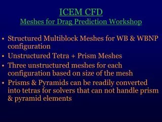
Available (Posted) Unstructured Grids • VGRID (NASA Langley) • Node-Based grids NASA(W1,W2,WB,WBF) • Node-Based grids Cessna (W1,W2) • Cell Centered Grids Raytheon (WB,WBF) • ANSYS Hybrid Meshes • Centaur (DLR, adapted) (Node Based) • AFLR3 (Boeing) (Cell Centered) • TAS (JAXA) (Node Based) • GridPro (Block-Structured/Unstructured)
VGRID NASA (Node Based) • WB: • Coarse : 5.3M pts • Medium: 14.3M pts • Fine: 40.0M pts (> 200M cells) • WBF: • Coarse: 5.6M pts • Medium: 14.6M pts • Fine: 41.1M pts ( > 200M cells)
NSU3D Description • Unstructured Reynolds Averaged Navier-Stokes solver • Vertex-based discertization • Mixed elements (prisms in boundary layer) • Edge data structure • Matrix artificial dissipation • Option for upwind scheme with gradient reconstruction • No cross derivative viscous terms • Thin layer in all 3 directions • Option for full Navier-Stokes terms
Solver Description (cont’d) • Spalart-Allmaras turbulence model • (original published form) • Optional k-omega model
Solution Strategy • Jacobi/Line Preconditioning • Line solves in boundary layer regions • Relieves aspect ratio stiffness • Agglomeration multigrid • Fast grid independent convergence rates • Parallel implementation • MPI/OpenMP hybrid model • DPW runs: MPI on local cluster and on NASA Columbia Supercomputer
Grid Generation • Runs based on NASA Langley supplied VGRIDns unstructured grids • Tetrahedra in Boundary Layer merged into prismatic elements • Grid sizes up to 41M pts, 240M elements
Sample Run Times • All runs performed on NASA Columbia Supercomputer • SGI Altix 512cpu machines • Coarse/Medium (~15Mpts) grids used 96 cpus • Using 500 to 800 multigrid cycles • 30 minutes for coarse grid • 1.5 hrs for medium grid • Fine Grids (~40M pts) used 248 cpus • Using 500 to 800 multigrid cycles • 1.5 to 2 hrs hrs for fine grid • CL driver and constant incidence convergence similar • WB cases hard to converge (not entirely steady)
Scalability • Near ideal speedup for 72M pt grid on 2008 cpus of NASA Columbia Machine (~10 minutes for steady-state solution)
NSU3D Sensitivity Studies • Sensitivity to Distance Function Calculation Method • Effect of Multi-Dimensional Thin-Layer versus Full Navier-Stokes Terms • Sensitivity to Levels of Artificial Dissipation
Sensitivity to Distance Function • All DPW3 Calculations done with Eikonal equation distance function
Sensitivity to Navier-Stokes Terms • All DPW3 Calculations done with Multidimensional Thin-Layer Formulation
Sensitivity to Dissipation Levels • Drag is grid converging • Sensitivity to dissipation decreases as expected • All Calculations done with low dissipation level
WBF Convergence (fixed alpha) • “Similar” convergence for all grids • Force coefficients well converged < 500 MG cycles
WBF Convergence • Medium Grid (15M pts): Fixed alpha
WBF Convergence • Medium Grid (15M pts): Fixed CL
WBF Convergence • Similar convergence (Fixed CL or alpha)
WBF: Grid Convergence Study • CP at wing break station (y/b=0.411)
WBF: Grid Convergence Study • CP at wing break station (y/b=0.411)
WBF: Grid Convergence Study • CP at wing break station (y/b=0.411)
WBF: Grid Convergence Study • CF at wing break station (y/b=0.411)
WBF: Grid Convergence Study • Good fairing design (coarse grid: 5M pts)
WBF: Grid Convergence Study • Good fairing design (medium grid: 15M pts)
WBF: Grid Convergence Study • Good fairing design (fine grid: 40M pts)
WBF: TE Separation • Coarse grid: 5M pts
WBF: Drag Polar • CP at wing break station (y/b=0.411)
WBF: Drag Polar • CP at wing break station (y/b=0.411)
WBF: Drag Polar • CP at wing break station (y/b=0.411)
WBF: Drag Polar • CP at wing break station (y/b=0.411)
WBF: Drag Polar • CP at wing break station (y/b=0.411)
WBF: Drag Polar • CP at wing break station (y/b=0.411)
WBF: Drag Polar • CP at wing break station (y/b=0.411)
WBF: Drag Polar • CP at wing break station (y/b=0.411)
WBF: Drag Polar • CP at wing break station (y/b=0.411)
WBF: Drag Polar • CFX at wing break station (y/b=0.411)
WBF: Drag Polar • Full Polar run on all 3 grids (5, 15, 40M pts)
WBF: Drag Polar • Full Polar run on all 3 grids (5, 15, 40M pts)
WBF: Moment • Full Polar run on all 3 grids (5, 15, 40M pts)
WBF: Moment • Full Polar run on all 3 grids (5, 15, 40M pts)
WB Convergence (fixed alpha) • Separated Flow, unsteady shedding pattern • Smaller residual excursions with fewer MG levels • Moderate CL variations
WB Medium Grid • Plot Min and Max unsteady CL values
WB Medium Grid • Plot Min and Max unsteady CL values • Good overlap in polar– suitable drag values
WB Medium Grid • Plot Min and Max unsteady CL values • Less overlap in CM