Download
1 / 82
830 likes | 998 Vues
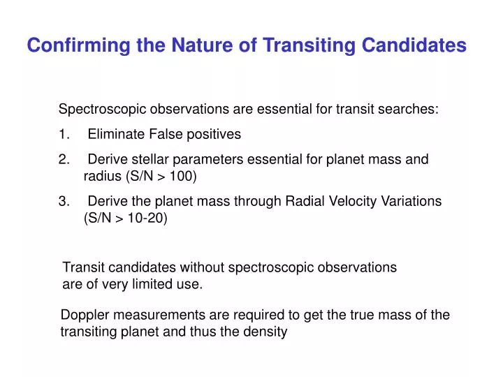
Confirming the Nature of Transiting Candidates. Spectroscopic observations are essential for transit searches: Eliminate False positives Derive stellar parameters essential for planet mass and radius (S/N > 100) Derive the planet mass through Radial Velocity Variations (S/N > 10-20).

E N D
Confirming the Nature of Transiting Candidates • Spectroscopic observations are essential for transit searches: • Eliminate False positives • Derive stellar parameters essential for planet mass and radius (S/N > 100) • Derive the planet mass through Radial Velocity Variations (S/N > 10-20) Transit candidates without spectroscopic observations are of very limited use. Doppler measurements are required to get the true mass of the transiting planet and thus the density
⅓ 1 ( 2pG Mp sin i ( P Ms⅔ (1 – e2)½ In general from Kepler‘s law: Mp = mass of planet Ms = mass of star P = orbital period K= For circular orbits (often the case for transiting Planets): Where Mp is in Jupiter masses, P is in years, and Ms is in solar masses Mp sin i 28.4 K= m/s P1/3Ms2/3
Radial Velocity Amplitude of Planets at Different a G2 V star Radial Velocity (m/s)
A0 V star Radial Velocity (m/s)
M2 V star Radial Velocity (m/s)
Cross disperser slit collimator Echelle Spectrographs camera detector corrector From telescope Echelle grating
∞ y l2 Dy dl Free Spectral Range Dl = l/m m-2 m-1 m m+2 m+3 Grating cross-dispersed echelle spectrographs
What does the radial velocity precision depend on? • The spectral resolution (≡ l/dl) • The Signal to Noise Ratio (S/N) of your data. • Your wavelength coverage: the more spectral lines the more radial velocity measurements you have • The type of star you are looking at
← 2 detector pixels dl l R = dl Spectral Resolution Consider two monochromatic beams They will just be resolved when they have a wavelength separation of dl Resolving power: dl = full width of half maximum of calibration lamp emission lines For Doppler confirmation of planets you need R = 50000 - 100000 l1 l2
How does the radial velocity precision depend on all parameters? s (m/s) = Constant × (S/N)–1 R–3/2 (Dl)–1/2 • : error R: spectral resolving power S/N: signal to noise ratio Dl : wavelength coverage of spectrograph in Angstroms For R=110.000, S/N=150, Dl=2000 Å, s = 2 m/s C ≈ 2.4 × 10¹¹ For a given instrument you can take its actual performance with real observations and scale accordingly
A7 star K0 star Early-type stars have few spectral lines (high effective temperatures) and high rotation rates.
v sin i ( ) 2 Including dependence on stellar parameters s (m/s) ≈ Constant ×(S/N)–1 R–3/2 (Dl)–1/2 f(Teff) v sin i : projected rotational velocity of star in km/s f(Teff) = factor taking into account line density f(Teff) ≈ 1 for solar type star f(Teff) ≈ 3 for A-type star f(Teff) ≈ 0.5 for M-type star For RV work the useful wavelength coverage is no more than 1000-2000 Å
For planet detection with radial velocity measurements you need a stable spectrograph. The traditional way of doing wavelength calibrations introduces instrumental errors. You need special tricks Observe your star→ Then your calibration source→ The classic method should work for RV amplitudes of more than 100 m/s
Because the calibration source is observed at a different time from your star you can have instrumental shifts ... Short term shifts of the spectrograph can limit precision to several hunrdreds of m/s
Stellar spectrum Thorium-Argon calibration Method 1: Observe your calibration source (Th-Ar) simultaneously to your data: Spectrographs: CORALIE, ELODIE, HARPS
Method 2: Iodine cell Spectrum of Iodine Spectrum of Iodine + Star
OGLE: 8 exoplanets V=14-15.8 Last discovery: 2007 Is doubtful that any more spectroscopic observations follow-up observations will be made of OGLE candidates because they are too faint. Groups will either observe Kepler/CoRoT targets (best possible light curves) or WASP/HAT candidates (bright) Transit Discoveries HAT: 31 exoplanets V=8.7-13.2 WASP: 66 exoplanets V=8.3-12.6 Kepler: 24 exoplanets V=11-14 CoRoT: 24 exoplanets V=11.7-16
RV error SOPHIE Period (days) RV Error/Amplitude V-magnitude In an ideal world with only photon noise: RV error HARPS and HIRES Jupiter Neptune RV error ESPRESSO (VLT) Superearth 7 (MEarth)
CoRoT-1b As a rule of thumb: if you have an RV precision less than one-half of the RV amplitude you need 8 measurements equally spaced in phase to detect the planet signal.
SOPHIE HARPS Time in hours required (on Target!) for the confirmation of a transiting planet in a 4 day orbit as a function of V-magnitude. RV measurement groups like bright stars!
Stellar activity can decrease your measurement precision !!! HD 166435 10 Radial Velocity (m/s) -10 0.4 0.6 0 0.2 0.8 Rotation Phase Radial velocity variations due entirely to spots
Stellar Activity can be the dominant noise source f is filling factor (photometric amplitude) in percent) vsini (V in figure) is rotational velocity in km/s Saar & Donahue (1996): ARV (m/s) = 6.5 f0.9 vsini f=0.5%, vsini=2 km/s → ARV = 7 m/s Hatzes (2001): ARV (m/s) = (8.6 vsini – 1.6) f0.9 f=0.5%, vsini=2 km/s → ARV = 8.3 m/s Two expressions agree to within 20%
Comparison of HARPS predicted RV error as a function of activity for a 10th magnitude star If you are looking at young active stars your RV precision will be signficantly worse and these will require more telescope resources In some cases it is possible to use „tricks“ to reduce the noise due to activity. See CoRoT-7b at end of lecture.
Curvature Span A Tool for confirming planets: Bisectors Bisectors can measure the line shapes and tell you about the nature of the RV variations: • What can change bisectors : • Spots • Blends • Pulsations
Correlation of bisector span with radial velocity for HD 166435: Spot
Spectroscopic binaries can also produce line profile changes
The Cross-Correlation Function (CCF) is a common way to measure the Radial Velocity of a Star: • The CCF of your observation can be taken with a template of a standard star, a mask (0 values in the continuum and 1 in spectral lines) or with one observation of your star (relative velocities). • The centroid of the CCF gives you the Radial Velocity • An assymetric CCF → blend • The CCF represents the mean shape of your spectral lines. Measuring the bisector of the CCF can reveal line shape variations In IRAF: rv package → fxcor
Confirming Transit Candidates Radial Velocity measurements are essential for confirming the nature (i.e. get the mass) of the companion, and to exclude so-called false postives: It looks like a planet, it smells like a planet, but it is not a planet • Grazing Eclipse by stellar companion • Giant Star eclipsed by a main sequence star • Background Eclipsing Binary (BEB) • Hiearchical Triple System • Star not suitable for radial velocity measurements • Unsolved cases
Before you start: Use what you know about transits! Transit phase = 0 If it is really a transiting/eclipsing body, then you expect the radial velocity to be zero at photometric (transit= phase zero, minimum at phase 0.25 and maximum at phase 0.75. RV variations must be in phase with the light curve.
OGLE-TR-3 is NOT a transiting planet. You know this immediately because the RV is not in phase with the transit
1. Grazing eclipse by a main sequence star: The shape of the light curve is the first indication of a binary star These are easy to exclude with Radial Velocity measurements as the amplitudes should be tens km/s (2–3 observations)
2. Giant Star eclipsed by main sequence star: Giant stars have radii of 10-100 Rsun. This results in an eclipse depth of 0.0001– 0.01 for a companion like the sun G star This scenario can be resolved with relatively little cost in telescope resources: • A longer than expected transit duration is the first hint that you have a large star. For example a transiting planet in a 10 day orbit will have a duration of 4 hrs. Around a 10 Rsun star (planet still outside of the star) the duration will be 39 hrs • A low resolution spectrum will establish the luminosity class of the star • Two radial velocity measurements taken at minimum and maximum will establish binarity
Low resolution spectra can easily distinguish between a giant and main sequence star for the host. This star was originally classified as a K0 main sequence star with photometry
CoRoT: LRa02_E2_2249 • Spectral Classification: • K0 III (Giant, spectroscopy) • Period: 27.9 d • Transit duration: 11.7 hrs → implies Giant, but long period! Mass ≈ 0.2 MSun
CoRoT: LRa02_E1_5015 • Spectral Classification: • K0 III (subgiant, photometry) • Period: 13.7 d • Transit duration: 10.1 hrs → Giant? Mass ≈ 0.2 MSun
3. Eclipsing Binary as a background (foreground) star: Fainter binary system in background or foreground Total = 17% depth Light from bright star Light curve of eclipsing system. 50% depth Difficult case. This results in no radial velocity variations as the fainter binary probably has too little flux to be measured by high resolution spectrographs. Large amounts of telescope time can be wasted with no conclusion. High resolution imaging may help to see faint background star.
4. Eclipsing binary in orbit around a bright star (hierarchical triple systems) Another difficult case. Radial Velocity Measurements of the bright star will show either long term linear trend no variations if the orbital period of the eclipsing system around the primary is long. This is essentialy the same as case 3) but with a bound system
CoRoT: LRa02_E1_5184 • Spectral Classification: • K1 V (spectroscopy) • Period: 7.4 d • Transit duration: 12.68 hrs • Depth : 0.56%
Bisector Radial Velocity Radial Velocity (km/s) Photometric Phase The Bisector variations correlate withthe RV → this is a blend s = 42 m/s Error: 20-30 m/s
5. Companion may be a planet, but RV measurements are impossible Period = Period: 4.8 d Transit duration: 5 hrs Depth : 0.67% No spectral line seen in this star. This is a hot star for which RV measurements are difficult
6. Sometimes you do not get a final answer Period: 9.75 Transit duration: 4.43 hrs Depth : 0.2% V = 13.9 Spectral Type: G0IV (1.27 Rsun) Planet Radius: 5.6 REarth Photometry: On Target The Radial Velocity measurements are inconclusive. So, how do we know if this is really a planet. CoRoT: LRc02_E1_0591 Note: We have over 30 RV measurements of this star: 10 Keck HIRES, 18 HARPS, 3 SOPHIE. In spite of these, even for V = 13.9 we still do not have a firm RV detection. This underlines the difficulty of confirmation measurements on faint stars.
LRa01_E2_0286 turns out to be a binary that could still have a planet But nothing is seen in the residuals