Download
1 / 52
3.41k likes | 8.5k Vues
ERTH2020 Introduction to Geophysics. The Electromagnetic (EM) Method Magnetotelluric (MT). Magnetotelluric. combination of magnetic and telluric* methods. (Latin ‘ tellūs ’ ‘earth’ “Earth current”). Magnetotelluric.

E N D
ERTH2020Introduction to Geophysics The Electromagnetic (EM) Method Magnetotelluric (MT)
Magnetotelluric combination of magnetic and telluric* methods (Latin ‘tellūs’ ‘earth’ “Earth current”)
Magnetotelluric …other scientists Tikhonov (1950) and Rikitake (1951), Kato & Kikuchi (1950).
Induction Equivalent Circuits I I I • DC Resistivity C L • Induced Polarisation R • Inductive EM
Goal 1. 1D diffusion equation 2. Skin Depth (Penetration Depth)
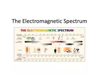
Contents Introduction Maxwell Equations Induction Sources Example EM theory Divergence & Curl Diffusion equation 1D Magnetotelluric Skin Depth Apparent Resistivity & Phase 2D MT Introduction Example
Electromagnetic Induction • Ampere’s Law (1826) • Faraday’s Law (1831) (magneto) quasi-static approximation , i.e. separation of electrical charges occur sufficiently slowly that the system can be taken to be in equilibrium at all times • electric current density (A/m2) • magnetic field intensity (A/m) • magnetic induction (Wb/m2 or T) • magnetic field intensity (V/m) e.g. http://farside.ph.utexas.edu/teaching/302l/lectures/node70.html http://farside.ph.utexas.edu/teaching/302l/lectures/node85.html
Electromagnetic Induction Simpson F. and Bahr K, 2005, p.18
Electromagnetic Induction Plane Wave Source • Faraday’s Law Primary field • Ampere’s Law • Ohm’s Law
Magnetotelluric Sources
Magnetotelluric Sources Power spectrum: signal's power (energy per unit time) falling within given frequency bins Simpson F. and Bahr K, 2005, p.3
Magnetotelluric Applications • Mineral exploration • Hydrocarbon exploration (oil/gas) • Deep crustal studies • Geothermal studies • Groundwater monitoring • Earthquake monitoring Simpson F. and Bahr K, 2005, p.3
Magnetotelluric Example 2D-MT resistivity model • Locations of MT measurement sites, Mount St Helens and nearby Cascades volcanoes. • White and red dots show the locations of the magnetotelluric measurements; measurement sites shown in red were used for 2D inversion. • The east–west line (red) shows the profile onto which these measurements were projected. The coloured area shows the region of high conductances. (=conductivity X thickness) • The green-to-orange transition corresponds to a conductance of 3000 Siemens. Hill et al., 2009
Magnetotelluric Example 2D-MT resistivity model after inversion the conductivity anomalies are caused by the presence of partial melt Hill et al., 2009
EM Theory gradient divergence curl (vector) (vector) (scalar)
Divergence (Interpretation) • The divergence measures how much a vector field ``spreads out'' or diverges from a given point, here (0,0): • Left: divergence > 0 since the vector field is ‘spreading out’ • Centre: divergence = 0 everywhere since the vectors are not spreading out. • Right: divergence < 0 since the vectors are coming closer together instead of spreading out. • is the extent to which the vector field flow behaves like a source or a sink at a given point. (If the divergence is nonzero at some point then there must be a source or sink at that position) http://citadel.sjfc.edu/faculty/kgreen/vector/block2/del_op/node5.html
Curl (Interpretation) • The curl of a vector field measures the tendency for the vector field to “swirl around”. (For example, let the vector field represents the velocity vectors of water in a lake. If the vector field swirls around, then when we stick a paddle wheel into the water, it will tend to spin.) • Left: curl > 0 (right-hand-rule thumb is up+) • Centre: curl = 0 everywhere since the field has no ‘swirling’. • Right: curl 0 since the vectors produce a torque on a test paddle wheel. • describes the infinitesimal rotation of a vector field ( p.s. The name "curl" was first suggested by James Clerk Maxwell in 1871) http://citadel.sjfc.edu/faculty/kgreen/vector/block2/del_op/node5.html & Wikipedia (Curl)
EM Theory Time-Domain Maxwell Equations (magneto-quasi-static) (Faraday) (Ampere) Also note that generally Note the use of the constitutive relations: first order, coupled PDEs
EM Theory Time-Domain Maxwell Equations (magneto-quasi-static) to uncouple, take the curl (Faraday) (Ampere) Second order, uncoupled PDEs
EM Theory Time-Domain Maxwell Equations (magneto-quasi-static) Second order, uncoupled PDEs Plane wave source sinusoidal time variation where the angular frequency and the imaginary unit • Complex numbers can also be written as • Compact way to describe waves • Complex numbers arise e.g. from equations such as. • Generally complex numbers have a real and imaginary part and are written as where is the real part and the imaginary part.
EM Theory Time-Domain Maxwell Equations (magneto-quasi-static) Second order, uncoupled PDEs Plane wave source sinusoidal time variation where the angular frequency and the imaginary unit • Complex numbers can also be written as • Compact way to describe waves • Complex numbers arise e.g. from equations such as. • Generally complex numbers have a real and imaginary part and are written as where is the real part and the imaginary part.
EM Theory Frequency Domain Diffusion Equations Second order, uncoupled PDEs General equations for inductive EM
EM Theory 1D solution with vector identity Diffusion Equations (Frequency Domain)
EM Theory 1D solution Divergence of Faraday’s law Divergence of Ampere’s law (Gauss law for magnetism, i.e. no magnetic monopoles) Proof via Cartesian coordinates
EM Theory 1D solution General solution for second-order PDE: decreases in amplitude with z increases in amplitude with z unphysical Simpson F. and Bahr K, 2005, p.21
EM Theory 1D solution Taking the second derivative with respect to z Real part Imaginary part Skin Depth (Penetration Depth) Simpson F. and Bahr K, 2005, p.22
EM Theory 1D solution Taking the second derivative with respect to z Real part Imaginary part Skin Depth (Penetration Depth) For angular frequency for a half-space with conductivity Simpson F. and Bahr K, 2005, p.22
EM Theory 1D solution Skin Depth (Penetration Depth) Simpson F. and Bahr K, 2005, p.22 & http://userpage.fu-berlin.de/~mtag/MT-principles.html
EM Theory 1D solution Real part Imaginary part The inverse of q is the Schmucker-WeideltTransfer Function ..has dimensions of length but is complex The Transfer Function C establishes a linear relationship between the physical properties that are measured in the field. Simpson F. and Bahr K, 2005, p.22
EM Theory 1D solution Schmucker-Weidelt Transfer Function We had with the general solution earlier However Faraday’s law is Therefore Simpson F. and Bahr K, 2005, p.22
EM Theory 1D solution Schmucker-Weidelt Transfer Function • is calculated from measured and fields (or and ) . • from the apparent resistivity can be calculated: apparent resistivity Simpson F. and Bahr K, 2005, p.22
EM Theory Apparent Resistivity and Phase apparent resistivity The phase is the lag between the E and H field and together with apparent resistivity one of the most important parameters in MT phase Simpson F. and Bahr K, 2005, p.22
EM Theory Apparent Resistivity and Phase For a homogeneous half space: • diagnostic of substrata in which resistivity increaseswith depth • diagnostic of substrata in which resistivity decreaseswith depth Simpson F. and Bahr K, 2005, p.26
EM Theory Simpson F. and Bahr K, 2005, p.27
2D-MT Introduction • For this 2-D case, EM fields can be decoupled into two independent modes: • E-fields parallel to strike with induced B-fields perpendicular to strike and in the vertical plane (E-polarisation or TE mode). • B-fields parallel to strike with induced E-fields perpendicular to strike and in the vertical plane (B-polarisationorTM mode). Simpson F. and Bahr K, 2005, p.27
2D-MT Introduction Simpson F. and Bahr K, 2005, p.30
2D solution TE-mode (E-Polarisation) Numerical Modelling in 2D • Numerical schemes, e.g.: • Finite Differences • Finite Elements EscriptFinite Element Solver (Geocomp UQ)
Numerical Modelling in 2D σ = 10-14 S/m σ = 0.1 S/m σ = 0.01 S/m Dirichlet boundary conditions via a single analytical 1D solution applied Left and Right; Top & Bottom via interpolation
Numerical Modelling in 2D Electric Field (Imaginary) Electric Field (Real)
Numerical Modelling in 2D Apparent Resistivity at selected station (all frequencies)
Numerical Modelling in 2D σ = 10-14 S/m σ = 0.04 S/m σ = 0.4 S/m σ = 0.1 S/m σ = 0.001 S/m # Zones = 71389 σ = 0.2 S/m # Nodes = 36343
Numerical Modelling in 2D Real Part Imaginary Part
Numerical Modelling in 2D Apparent Resistivity f = 1 Hz r = 25 Ωm r = 2.5 Ωm r = 10 Ωm Skin-depth r = 1000 Ωm r = 2 Ωm
References Simpson F. and Bahr K.: “Practical magnetotellurics”, 2005, Cambridge University Press Cagniard, L. (1953) Basic theory of the magneto-telluric method of geophysical prospecting, Geophysics, 18, 605–635 Hill G J., Caldwell T.G, Heise W., Chertkoff D.G., Bibby H.M., Burgess M.K., Cull J.P., Cas R.A.F.: "Distribution of melt beneath Mount St Helens and Mount Adams inferred from magnetotelluric data", Nature Geosci., 2009, V2, pp.785
EM Theory (Faraday) (Gauss law for magnetism) via Cartesian coordinates
EM Theory (Ampere) however, the rate of change of the charge density ρequals the divergence of the current density J Continuity equation (Gauss law)