Distribution of Estimates and Multivariate Regression
250 likes | 384 Vues
This lecture on multivariate regression delves into the distribution of estimates and the underlying distributional assumptions. It discusses the conditional normal model, likelihood functions, and how least squares estimators align with maximum likelihood estimators when error terms are normal. The variance of estimator parameters is derived from the Gauss-Markov theorem, and matrix representations of multivariate models are introduced. Important relationships, including variances and estimators, are presented to solidify understanding of the multivariate approach in regression analysis.

Distribution of Estimates and Multivariate Regression
E N D
Presentation Transcript
Distribution of Estimates and Multivariate Regression Lecture XXIX
Models and Distributional Assumptions • The conditional normal model assumes that the observed random variables are distributed • Thus, E[yi|xi]=a+bxi and the variance of yi equals s2. The conditional normal can be expressed as
Further, the ei are independently and identically distributed (consistent with our BLUE proof). • Given this formulation, the likelihood function for the simple linear model can be written:
Taking the log of this likelihood function yields: • As discussed in Lecture XVII, this likelihood function can be concentrated in such a way so that
So that the least squares estimator are also maximum likelihood estimators if the error terms are normal. • Proof of the variance of b can be derived from the Gauss-Markov results. Note from last lecture:
Remember that the objective function of the minimization problem that we solved to get the results was the variance of estimate:
This assumes that the errors are independently distributed. Thus, substituting the final result for di into this expression yields:
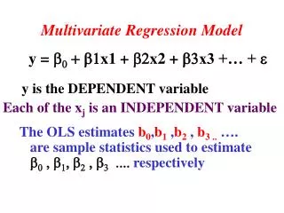
Multivariate Regression Models • In general, the multivariate relationship can be written in matrix form as:
If we expand the system to three observations, this system becomes:
In matrix form this can be expressed as • The sum of squared errors can then be written as:
A little matrix calculus is a dangerous thing • Note that each term on the left hand side is a scalar. Since the transpose of a scalar is itself, the left hand side can be rewritten as:
Variance of the estimated parameters • The variance of the parameter matrix can be written as:
Substituting this back into the variance relationship yields:
Theorem 12.2.1 (Gauss-Markov) Let b*=C’y where C is a T x K constant matrix such that C’X=I. Then, b^is better than b* if b* ≠ b^.
This choice of C guarantees that the estimator b* is an unbiased estimator of b. The variance of b* can then be written as:
To complete the proof, we want to add a special form of zero. Specifically, we want to add s2(X’X)-1-s2(X’X)-1=0.
Focusing on the last terms, we note that by the orthogonality conditions for the C matrix
Focusing on the last terms, we note that by the orthogonality conditions for the C matrix
The minimum variance estimator is then C=X(X’X)-1 which is the ordinary least squares estimator.